Qubit-Wise Commutativity: A Practical Guide to Quantum Measurement Optimization for Biomedical Research

Abstract

This article provides a comprehensive exploration of qubit-wise commutativity (QWC) and its critical role in optimizing quantum measurements for variational algorithms like the Variational Quantum Eigensolver (VQE). Aimed at researchers, scientists, and drug development professionals, we cover the foundational theory of QWC versus full commutativity, demonstrate practical implementation using modern quantum libraries, address common troubleshooting scenarios, and present a comparative analysis of grouping strategies. By reducing the number of required quantum measurements by up to 90%, these techniques offer a practical path to overcoming a major bottleneck in applying quantum computing to molecular simulation and drug discovery on near-term hardware.

Understanding the Quantum Measurement Problem and Qubit-Wise Commutativity Fundamentals

The Quantum Measurement Bottleneck in NISQ Algorithms

The Noisy Intermediate-Scale Quantum (NISQ) era is defined by quantum processors containing from approximately 50 to 1000 qubits that operate without the benefit of full quantum error correction [1] [2]. These devices are characterized by high error rates, limited coherence times, and gate fidelities that restrict executable circuit depths to roughly 1,000 operations before noise overwhelms the computational signal [2]. Within this constrained environment, Variational Quantum Algorithms (VQAs) have emerged as a leading algorithmic paradigm, particularly for quantum chemistry and drug discovery applications [1] [3]. However, the efficient estimation of molecular observables—a computational primitive fundamental to these applications—presents a critical bottleneck [4]. The core of this bottleneck lies in the measurement overhead required for Hamiltonian expectation value estimation, which scales as O(N⁴) to O(N⁸) for problems of interest, potentially requiring millions of state preparations to achieve chemical accuracy [4]. This article examines the quantum measurement bottleneck, the recent advances in measurement grouping strategies—with a specific focus on qubit-wise commutativity—and the experimental methodologies enabling progress toward practical quantum advantage in computational chemistry and drug development.

The Fundamental Challenge of Observable Estimation

Mathematical Foundation of the Measurement Problem

In quantum chemistry simulations on NISQ devices, the target observable is typically a molecular Hamiltonian H, which must be decomposed into a linear combination of N-qubit Pauli operators (tensor products of Pauli matrices X, Y, Z, and the identity I) [4]:

[H = \sum{i=1}^{M} ci Pi, \quad \text{where } Pi = \bigotimes{j=1}^{N} \sigma{ij}, \ \sigma{ij} \in {X, Y, Z, I}, \ ci \in \mathbb{R}]

The expectation value (\langle \psi | H | \psi \rangle) for a quantum state (|\psi\rangle) is approximated through quantum measurement. For each Pauli term (Pi), the quantum computer prepares the state and measures it to construct an estimator (\hat{Pi}) [4]. The fundamental challenge arises because each Pauli term may require a different measurement basis, and the number of terms M grows rapidly with system size. Direct sequential measurement of each term would be prohibitively expensive in terms of quantum resources [4].

Impact on Algorithmic Performance

The measurement bottleneck directly impacts the feasibility and efficiency of NISQ algorithms for drug discovery. The Variational Quantum Eigensolver (VQE), widely used for molecular ground state energy calculations, relies on repeated estimation of the Hamiltonian expectation value during its optimization loop [1] [3]. The excessive measurement overhead can render chemically accurate calculations impractical even for small molecules, limiting the scale of quantum chemistry problems addressable on current hardware [4]. This constraint is particularly acute for pharmaceutical applications where studying complex molecular interactions requires precise energy calculations beyond the capabilities of classical computers.

Measurement Grouping Strategies: From Full Commutation to Qubit-Wise Commutativity

Foundations of Simultaneous Measurement

To reduce measurement overhead, simultaneous measurement strategies group multiple Pauli operators that can be measured using the same quantum circuit and measurement basis [4]. Two primary grouping schemes have been developed:

• Fully Commuting (FC) Groups: Operators that commute according to the standard commutation relation ([Pi, Pj] = PiPj - PjPi = 0) can be simultaneously diagonalized and measured [4]. While FC grouping provides the lowest estimator variance, it requires entangling operations for diagonalization that introduce significant noise and potential bias on NISQ devices [4].

• Qubit-Wise Commuting (QWC) Groups: A stricter commutativity relation where two Pauli operators commute if their corresponding single-qubit Pauli operators commute at every qubit position [4]. While QWC groups exhibit higher variance than FC groups, they can be measured with single-qubit basis rotations without entangling gates, making them more noise-resilient on NISQ devices [4].

Table 1: Comparison of Pauli Grouping Strategies for Molecular Hamiltonian Measurement

Grouping Strategy	Commutation Relation	Circuit Requirements	Noise Resilience	Estimator Variance
Full Commutation (FC)	([Pi, Pj] = 0)	Requires entangling gates for diagonalization	Low (high bias from noise)	Lowest
Qubit-Wise Commutation (QWC)	Commutes at every qubit position	Single-qubit rotations only	High (minimal bias)	Higher than FC
GALIC (Hybrid)	Context-aware interpolation	Selective entangling gates	Adaptive to device noise	20% lower than QWC

Qubit-Wise Commutativity: Formal Definition and Significance

Qubit-wise commutativity represents a hardware-efficient alternative to full commutativity that has been widely adopted in quantum software packages [4]. Formally, two N-qubit Pauli operators (P = \bigotimes{k=1}^{N} \sigmak) and (Q = \bigotimes{k=1}^{N} \tauk) are qubit-wise commuting if for every qubit position k, the single-qubit Pauli operators (\sigmak) and (\tauk) commute: (\sigmak \tauk = \tauk \sigmak) for all k = 1, ..., N [4].

This relation is strictly stronger than full commutativity—all QWC operators are fully commuting, but not all fully commuting operators are QWC. The practical significance for NISQ algorithms lies in the measurement circuit simplicity: QWC groups can be diagonalized using only single-qubit gates rather than entangling operations, significantly reducing circuit depth and noise susceptibility [4]. This makes QWC particularly valuable for pharmaceutical applications where measurement reliability may outweigh the additional state preparation cost.

Figure 1: Logical relationships between Pauli measurement grouping strategies, highlighting the trade-offs between different approaches for NISQ algorithms.

Advanced Hybrid Frameworks: Interpolating Between FC and QWC

The GALIC Framework: Generalized Backend-Aware Pauli Commutation

The Generalized backend-Aware pauLI Commutation (GALIC) framework represents a significant advancement by providing a systematic approach to interpolate between FC and QWC grouping strategies [4] [5]. GALIC introduces a context-aware hybrid commutativity relation that dynamically adjusts grouping strategy based on device characteristics including noise levels, connectivity, and gate fidelities [4]. This approach recognizes that the binary choice between FC and QWC is suboptimal—instead, selective introduction of entangling gates in a noise-aware manner can achieve better variance characteristics than QWC while maintaining higher fidelity than FC [4].

Performance Advantages of Hybrid Grouping

Experimental results demonstrate that GALIC achieves a 20% average reduction in estimator variance compared to QWC while maintaining chemical accuracy (error < 1 kcal/mol) [4] [5]. Furthermore, hardware experiments on IBM quantum processors show 1.2× lower GALIC estimator variance compared to QWC, validating numerical simulations [4]. This performance improvement is achieved without introducing excessive bias from noisy entangling operations, striking an optimal balance for NISQ devices.

Table 2: Quantitative Performance Comparison of Grouping Strategies on Molecular Hamiltonians

Molecule (Qubits)	Grouping Strategy	Estimator Variance	Measurement Overhead	Energy Error (kcal/mol)
Hâ‚‚ (4)	QWC	1.00 (baseline)	1.00 (baseline)	0.45
	FC	0.72	0.75	0.52
	GALIC	0.80	0.82	0.47
LiH (12)	QWC	1.00 (baseline)	1.00 (baseline)	0.78
	FC	0.68	0.71	0.85
	GALIC	0.79	0.81	0.74
Hâ‚‚O (14)	QWC	1.00 (baseline)	1.00 (baseline)	0.92
	FC	0.65	0.69	1.12
	GALIC	0.76	0.78	0.89

Experimental Protocols and Methodologies

Benchmarking Framework for Grouping Strategies

Rigorous evaluation of measurement grouping strategies requires a standardized benchmarking approach:

• Hamiltonian Selection: Test on a series of molecular Hamiltonians of increasing complexity (from Hâ‚‚ to Hâ‚‚O) generated through classical electronic structure codes [4].

• Device Modeling: Implement realistic noise models based on characterized quantum hardware (e.g., IBM and IonQ processors) including gate infidelities, coherence times, and measurement errors [4].

• Grouping Algorithm Application: Apply FC, QWC, and hybrid grouping algorithms to the Hamiltonian terms, recording the number of groups and estimated measurement costs [4].

• Variance Estimation: For each grouping strategy, compute the estimator variance as (\text{Var}[\hat{H}] = \sum{i=1}^{M} |ci|^2 \text{Var}[\hat{Pi}] / ni), where (n_i) is the number of measurements allocated to group i [4].

• Bias Evaluation: Quantify estimator bias introduced by noisy entangling operations in FC groups through comparison with noiseless simulations [4].

Hardware-Aware Optimization Protocol

The GALIC framework implements a specialized experimental protocol for device-aware optimization:

• Device Characterization: Profile target quantum processor for qubit-specific error rates, connectivity constraints, and two-qubit gate fidelities [4].

• Connectivity-Aware Grouping: Form initial QWC groups, then selectively merge groups using FC relations only when the required entangling operations can be implemented efficiently given device connectivity [4].

• Noise-Adaptive Diagonalization: Design measurement circuits that minimize depth and maximize fidelity by exploiting device-specific native gate sets and connectivity [4].

• Dynamic Resource Allocation: Allocate measurement shots across groups proportional to both coefficient magnitude (|c_i|) and group variance, with adjustments for device-specific error rates [4].

Figure 2: Experimental workflow for hardware-aware measurement grouping, showing the sequence from Hamiltonian decomposition through to energy estimation with device-specific optimizations.

Table 3: Research Reagent Solutions for Quantum Measurement Optimization Studies

Resource/Tool	Function	Example Implementation
Quantum Chemistry Packages	Generate molecular Hamiltonians as Pauli sums	OpenFermion, PSI4, PySCF
Grouping Algorithms	Partition Pauli terms into measurable groups	GALIC [4], Sorted Insertion [4]
Device Noise Models	Simulate realistic hardware behavior	IBM Qiskit Noise Models, Cirq Noise
Variance Estimation Tools	Predict measurement overhead	Custom estimators based on (\sum	c_i	^2 \text{Var}[\hat{Pi}]/ni) [4]
Error Mitigation Techniques	Reduce bias from noisy operations	Zero-noise extrapolation, symmetry verification [1]
Hardware Benchmarks	Validate grouping strategies on real devices	IBM Quantum, IonQ, Quantinuum [6]

Implications for Pharmaceutical Research and Beyond

The development of advanced measurement grouping strategies has significant implications for quantum chemistry applications in pharmaceutical research. By reducing the measurement overhead by over 20% compared to standard QWC approaches [4], hybrid frameworks like GALIC bring chemically accurate quantum computations closer to practicality on NISQ devices. This enhancement is particularly valuable for drug discovery pipelines, where efficient calculation of molecular interaction energies and reaction barriers could accelerate screening of candidate compounds.

Furthermore, the research reveals that error suppression has a 13× larger impact on device-aware estimator variance than qubit connectivity [4] [5], suggesting that improving gate fidelity may be more critical than expanding qubit connectivity for near-term quantum advantage in pharmaceutical applications. This insight directs hardware development priorities toward error reduction rather than architectural complexity.

The quantum measurement bottleneck represents a fundamental challenge for practical quantum chemistry on NISQ devices. While qubit-wise commutativity provides a noise-resilient foundation for measurement grouping, emerging hybrid frameworks like GALIC demonstrate that context-aware interpolation between FC and QWC strategies can significantly reduce measurement overhead while maintaining accuracy. For pharmaceutical researchers leveraging quantum computations, these advances in measurement optimization translate directly to expanded problem sizes, improved accuracy, and reduced computational costs. As quantum hardware continues to evolve with improvements in both scale and fidelity, sophisticated measurement strategies will remain essential for extracting maximal computational power from NISQ devices for drug discovery applications.

In quantum mechanics, the concept of commutativity serves as a fundamental indicator of the relationship between physical observables and the mathematical structure of the theory. The commutator of two operators, defined as $[A,B] = AB - BA$, provides a precise mathematical framework for determining whether two observables can be simultaneously measured with arbitrary precision [7] [8]. When $[A,B] = 0$, the operators commute, indicating the existence of a common set of eigenstates and the possibility of simultaneous measurement without mutual disturbance [9] [10]. The physical significance of the commutator extends beyond a mere mathematical construct; it encodes essential information about how the measurement of one observable affects the state of a system when followed by measurement of another observable [11].

In the context of quantum computation and specifically measurement grouping algorithms, understanding commutativity—particularly specialized forms like qubit-wise commutativity—becomes crucial for optimizing resource utilization and reducing measurement overhead [12]. This technical guide explores the mathematical foundations of commutativity, its physical interpretations, and its practical applications in quantum computing, with particular emphasis on its role in measurement reduction techniques for variational quantum algorithms.

Mathematical Foundations of Commutativity

Basic Definitions and Properties

In quantum mechanics, physical observables are represented by self-adjoint operators acting on a Hilbert space [7]. The commutator of two operators $A$ and $B$ is defined as:

$$[A, B] = AB - BA$$

This mathematical object possesses several important algebraic properties [8]:

• Anticommutativity: $[A, B] = -[B, A]$
• Bilinearity: $[aA + bB, C] = a[A, C] + b[B, C]$ for scalars $a, b$
• Product Rule: $[A, BC] = [A, B]C + B[A, C]$
• Jacobi Identity: $[A, [B, C]] + [B, [C, A]] + [C, [A, B]] = 0$

These properties establish the commutator as a fundamental algebraic structure in quantum theory.

Complete Sets of Commuting Observables (CSCO)

A complete set of commuting observables (CSCO) refers to a set of mutually commuting operators whose common eigenvectors can be used as a basis to express any quantum state [9]. For operators with discrete spectra, a CSCO is a set of commuting observables whose simultaneous eigenspaces span the Hilbert space with linearly independent eigenvectors that are uniquely specified by corresponding sets of eigenvalues [9].

The significance of CSCOs lies in their ability to provide a unique labeling of quantum states. When degeneracy exists in the energy spectrum alone, additional commuting observables are needed to distinguish between eigenstates [9]. For instance, in the case of the hydrogen atom, the Hamiltonian exhibits degeneracy, requiring additional quantum numbers ($n$, $l$, $ml$, $ms$) corresponding to commuting observables to fully specify the state.

Table 1: Examples of Commuting and Non-Commuting Observables

Commuting Observables	Non-Commuting Observables	Commutator Value
Position components ($x$, $y$, $z$)	Position and momentum in same direction ($x$, $p_x$)	$[\hat{x}, \hat{p}_x] = i\hbar$
Momentum components ($px$, $py$, $p_z$)	Different components of angular momentum ($Lx$, $Ly$)	$[Lx, Ly] = i\hbar L_z$
Hamiltonian and parity in symmetric systems	Position and kinetic energy	Non-zero

Physical Interpretation of Commutativity

Measurement Compatibility

The physical significance of commutativity becomes apparent when considering quantum measurements. Two observables $A$ and $B$ are compatible (can be measured simultaneously) if and only if their commutator vanishes: $[A, B] = 0$ [11] [10]. This mathematical condition ensures the existence of a common eigenbasis ${|u_n\rangle}$ such that:

$$\hat{A}|u{n}\rangle=an|u{n}\rangle$$ $$\hat{B}|u{n}\rangle=bn|u{n}\rangle$$

When two observables commute, measuring one does not disturb the eigenstate of the other [10]. If a system is prepared in a common eigenstate $|ui\rangle$ of both operators, measuring $A$ yields $ai$ with certainty, and subsequently measuring $B$ yields $bi$ with certainty, with the state remaining unchanged as $|ui\rangle$ throughout the process [10].

Commutativity and Disturbance

For non-commuting observables ($[A, B] \neq 0$), the measurement process introduces fundamental disturbances. The commutator $[A,B]$ quantifies the extent to which the action of $B$ changes the value of the dynamical variable $A$, and vice versa [11]. This relationship is formally captured in generalized uncertainty principles, which establish fundamental limits on the precision with which incompatible observables can be simultaneously known [7].

The most famous example of non-commutativity is the position-momentum uncertainty relation, derived from $[\hat{x}, \hat{p}] = i\hbar$, which leads to the Heisenberg uncertainty principle $\Delta x \Delta p \geq \hbar/2$ [8]. This non-commutativity fundamentally distinguishes quantum mechanics from classical physics.

Figure 1: Measurement outcomes based on commutativity of observables

Commutativity in Quantum Computation

Qubit-Wise Commutativity and Measurement Grouping

In quantum computing, particularly for variational quantum algorithms like the Variational Quantum Eigensolver (VQE), measurement reduction through operator grouping is essential for practical implementation [12]. Two primary grouping schemes have been developed:

• Full commutativity (FC): Operators commute according to the standard definition $[A,B] = 0$
• Qubit-wise commutativity (QWC): A stricter condition where operators commute component-wise on each qubit

Qubit-wise commutativity represents a special case where Pauli operators act on different qubits or identical Pauli operators act on the same qubits [12]. This form of commutativity is particularly valuable in near-term quantum devices as it enables simultaneous measurement with minimal circuit overhead.

Recent research has introduced hybrid approaches, such as the GALIC framework (Generalized backend-Aware pauLI Commutation), which interpolates between FC and QWC to optimize measurement efficiency while accounting for device-specific noise characteristics and connectivity constraints [12]. These advanced commutativity relations can reduce estimator variance by an average of 20% compared to standard QWC approaches [12].

Mathematical Formulation of Qubit-Wise Commutativity

For multi-qubit systems, quantum states are described using tensor product spaces. The general state of an n-qubit system can be expressed as:

$$|\psi\rangle = \sum{i1,i2,...,in \in {0,1}} a{i1i2...in}|i1\rangle \otimes |i2\rangle \otimes \cdots \otimes |i_n\rangle$$

where the complex coefficients satisfy the normalization condition $\sum |a{i1i2...in}|^2 = 1$ [13].

In this context, qubit-wise commutativity imposes that for two operators $A$ and $B$, composed of tensor products of single-qubit operators:

$$A = \bigotimes{k=1}^n Ak, \quad B = \bigotimes{k=1}^n Bk$$

the condition $[Ak, Bk] = 0$ must hold for all qubits $k = 1, \ldots, n$. This ensures that measurements can be performed independently on each qubit without mutual disturbance.

Table 2: Commutativity Types in Quantum Measurement Grouping

Commutativity Type	Mathematical Condition	Measurement Implications	Resource Requirements
Full Commutativity (FC)	$[A,B] = AB - BA = 0$	Can be measured simultaneously	May require entangling gates for measurement
Qubit-Wise Commutativity (QWC)	$[Ak, Bk] = 0$ for all qubits $k$	Can be measured with single-qubit operations	Minimal overhead, suitable for NISQ devices
k-Commutativity	Intermediate between FC and QWC	Balanced trade-off between measurements and circuit depth	Adaptive based on device constraints

Figure 2: Hierarchy of commutativity relations in quantum measurement

Advanced Commutativity Concepts

Generalized Measurement and POVMs

In generalized quantum measurement theory, projective measurements are extended to Positive Operator-Valued Measures (POVMs) [7]. A POVM is a set of positive semi-definite operators ${F_i}$ that sum to the identity:

$$\sum{i=1}^n Fi = I$$

The probability of obtaining outcome $i$ when measuring state $\rho$ is given by $\text{Prob}(i) = \text{tr}(\rho F_i)$ [7].

POVMs generalize projective measurements and allow for the description of measurement effects on subsystems. The commutativity concepts extend to POVMs, where commuting POVMs represent compatible measurements that can be performed simultaneously without disturbance.

State-Dependent and Return Value Commutativity

Beyond the standard commutativity definitions, more refined concepts have been developed for specific applications:

State-dependent commutativity recognizes that certain operations may commute only when applied to specific quantum states [14]. Formally, two operations $p$ and $q$ on the same object are commutative in object state $\sigma$ if for all possible sequences of operations $\omega$, the return parameters in the concatenated sequence $pq\omega$ applied to state $\sigma$ are identical to those in the sequence $qp\omega$ applied to $\sigma$ [14].

Return value commutativity extends this concept by considering operation executions including their return values, not just their input parameters [14]. This approach enables more nuanced commutativity relations that can enhance concurrency in quantum and classical distributed systems.

Experimental Protocols and Research Toolkit

Methodology for Commutativity Verification

Experimental verification of commutativity relationships in quantum systems follows these key protocols:

• State Preparation: Initialize the system in a known state $|\psi\rangle$
• Sequential Measurement: Measure $A$ followed by $B$ on multiple identical preparations
• Reverse Sequence: Measure $B$ followed by $A$ on a fresh set of preparations
• Comparison: Statistically compare outcome distributions for the two sequences
• Commutation Test: If the measurement statistics are identical within experimental error, the operators commute

For multi-qubit systems, this procedure is extended to verify qubit-wise commutativity by testing component operations on individual qubits.

Research Reagent Solutions for Commutativity Studies

Table 3: Essential Research Tools for Commutativity and Measurement Studies

Research Tool	Function	Application Context
Variational Quantum Eigensolver (VQE)	Hybrid quantum-classical algorithm for ground state energy estimation	Quantum chemistry simulations [12]
Pauli Operator Sets	Tensor products of Pauli matrices ($X, Y, Z, I$)	Observable representation in quantum systems [12]
GALIC Framework	Generalized backend-Aware pauLI Commutation	Adaptive measurement grouping [12]
Quantum State Tomography	Complete characterization of quantum states	Verification of state preservation under commutative measurements
Randomized Measurement Protocols	Efficient estimation of multiple observables	Scalable verification of commutativity relations [12]
Tioxaprofen	Tioxaprofen, CAS:40198-53-6, MF:C18H13Cl2NO3S, MW:394.3 g/mol	Chemical Reagent
Talatisamine	Talatisamine, MF:C24H39NO5, MW:421.6 g/mol	Chemical Reagent

Commutativity serves as a fundamental organizing principle in quantum mechanics, with profound implications for both foundational theory and practical applications in quantum computing. From the basic mathematical definition $[A,B] = AB - BA$ to specialized forms like qubit-wise commutativity, this concept enables the classification of observables based on their mutual measurability.

In the context of quantum computation, particularly for measurement grouping in variational algorithms, understanding the hierarchy of commutativity relations—from full commutativity through k-commutativity to qubit-wise commutativity—provides essential tools for optimizing resource utilization on near-term quantum devices. Advanced frameworks like GALIC demonstrate how device-aware commutativity relations can significantly reduce measurement overhead while maintaining estimation accuracy.

As quantum hardware continues to advance, the refinement of commutativity concepts and their application to measurement reduction will play an increasingly important role in enabling practical quantum advantage for computational problems in chemistry, materials science, and optimization.

In the Noisy Intermediate-Scale Quantum (NISQ) era, efficient measurement of observables represents one of the most significant bottlenecks in variational quantum algorithms such as the Variational Quantum Eigensolver (VQE). The molecular Hamiltonians central to quantum chemistry applications are typically expressed as linear combinations of hundreds or even thousands of Pauli terms, creating a substantial measurement challenge [15]. Within this context, the strategic grouping of compatible observables has emerged as a crucial optimization technique, with qubit-wise commutativity (QWC) and full commutativity (FC) representing two fundamental approaches with distinct trade-offs [12] [16].

This technical guide examines the critical distinction between these commutativity paradigms, providing researchers and drug development professionals with a comprehensive framework for optimizing quantum measurements. The distinction is not merely theoretical; it directly impacts measurement efficiency, circuit depth, and ultimately the feasibility of quantum simulations on current hardware. We explore the mathematical foundations, practical implementations, and performance characteristics of both approaches, enabling informed selection based on specific research constraints and objectives.

Mathematical Foundations and Definitions

The Measurement Problem in Quantum Algorithms

Quantum algorithms for electronic structure determination, particularly VQE, estimate molecular ground state energies by measuring the expectation value of a qubit Hamiltonian ( H ), expressed as: [ H = \sum{i} ci hi ] where ( hi ) are Pauli strings (tensor products of Pauli operators ({I, \sigmax, \sigmay, \sigmaz})) and ( ci ) are real coefficients [15]. The expectation value ( \langle H \rangle ) is obtained by measuring each term individually: [ \langle H \rangle = \sumi ci \langle h_i \rangle ] For complex molecules, the number of terms can grow dramatically—from 15 for H₂ to 1,086 for H₂O in one example [15]—making naïve measurement approaches prohibitively expensive.

Commutativity in Quantum Mechanics

In quantum mechanics, two observables ( A ) and ( B ) are said to commute if their commutator vanishes: ([A, B] = AB - BA = 0). Commuting operators share a common set of eigenvectors and can be measured simultaneously without disturbing each other's measurement outcomes [7] [17]. This fundamental principle enables the grouping of multiple compatible observables into a single measurement circuit.

Formal Definitions of QWC and FC

Table: Comparison of Commutativity Types for Pauli Strings P and Q

Commutativity Type	Mathematical Definition	Physical Interpretation	Clifford Circuit Requirements
Full Commutativity (FC)	([P, Q] = PQ - QP = 0)	Operators commute as a whole	Multi-qubit entangling Clifford gates ((O(n^2/\log n)) depth) [16]
Qubit-Wise Commutativity (QWC)	([pi, qi] = 0) for all qubits (i)	Operators commute on every qubit individually	Single-qubit Clifford gates (depth-1 circuit) [16]

Full Commutativity (FC) represents the standard, mathematical notion of commutativity. Two Pauli strings ( P ) and ( Q ) fully commute if their product commutes regardless of their structure [16]. FC groups can be simultaneously measured using a Clifford unitary ( U ) that diagonalizes the entire set, but this transformation may require substantial quantum circuit depth—up to ( O(n^2/\log n) ) Clifford gates for ( n )-qubit systems [16].

Qubit-Wise Commutativity (QWC) imposes a stricter condition: Pauli strings ( P = \bigotimes{i=1}^n pi ) and ( Q = \bigotimes{i=1}^n qi ) qubit-wise commute if, for every qubit ( i ), the single-qubit Pauli operators ( pi ) and ( qi ) commute [16]. This stronger condition ensures that measurements can be performed using only single-qubit basis rotations (depth-1 circuits), but typically results in a larger number of measurement groups compared to FC.

The diagram above illustrates the logical relationship between QWC and FC. Critically, QWC implies FC (all qubit-wise commuting operators fully commute), but the converse is not necessarily true [16]. This hierarchy has profound implications for measurement efficiency.

Methodologies and Experimental Protocols

Grouping Algorithms and Strategies

Multiple algorithmic approaches exist for grouping Pauli terms into measurable fragments:

• QWC Grouping: Typically implemented using graph coloring algorithms where each Pauli term represents a vertex, with edges connecting non-commuting terms. The resulting graph coloring corresponds to measurement groups [17].

• FC Grouping: Leverages the full commutativity relation, often employing more complex grouping algorithms that account for the full commutator structure rather than individual qubit operations [12].

• Greedy Grouping: A practical approach that sequentially builds groups by selecting the largest ungrouped terms first, empirically producing fragments with varying variances that can reduce the sum of variance square roots [18].

• Overlapping Grouping: An advanced technique allowing Pauli products to appear in multiple groups, exploiting their compatibility with different measurement contexts to further reduce measurement counts [18].

Measurement and Estimation Protocols

The general workflow for efficient Hamiltonian measurement involves:

• Hamiltonian Preparation: Generate the qubit Hamiltonian through fermion-to-qubit mapping (e.g., Jordan-Wigner or Bravyi-Kitaev transformations) [15].

• Commutativity Analysis: Identify commuting subsets using either QWC or FC criteria based on hardware constraints and efficiency targets.

• Group Formation: Apply grouping algorithms (graph coloring, greedy, or overlapping methods) to partition the Hamiltonian into measurable fragments.

• Circuit Implementation: For each group, implement the appropriate diagonalizing circuit:

  • QWC: Single-qubit rotations to the Z-basis
  • FC: Multi-qubit Clifford circuits potentially requiring entangling gates

• Measurement Allocation: Distribute measurement shots optimally across groups, typically proportional to the variance of each fragment [18].

• Expectation Value Estimation: Compute ( \langle H \rangle = \sum\alpha \langle A\alpha \rangle ) from the grouped measurements, where ( A_\alpha ) represents each measurable fragment.

Quantitative Performance Analysis

Empirical Comparison of Grouping Strategies

Recent research provides quantitative comparisons of various grouping approaches across molecular systems:

Table: Estimator Variances for Different Molecules and Grouping Strategies (Data from Yen et al. 2023 [18])

Molecular System	LF Algorithm	Sorted Insertion (SI)	IMA	GMA	ICS
Hâ‚‚	0.136	0.136	0.136	0.136	0.136
LiH	5.84	2.09	1.73	1.52	0.976
BeHâ‚‚	14.3	6.34	5.60	5.26	4.29
Hâ‚‚O	116	48.2	-	-	-

The table demonstrates that advanced grouping strategies (IMA, GMA, ICS) consistently outperform simpler approaches (LF, SI), with the most flexible methods achieving the lowest estimator variances. This variance reduction directly translates to fewer required measurements for a target accuracy.

Resource Requirements and Trade-offs

Table: Resource Comparison Between QWC and FC Grouping Strategies

Resource Metric	QWC Grouping	FC Grouping	Hybrid Approaches
Number of Groups	Higher	Lower (up to 90% reduction vs. no grouping [15])	Intermediate
Circuit Depth	Shallow (depth-1 [16])	Deeper ((O(n^2/\log n)) Cliffords [16])	Configurable
Classical Overhead	Moderate	Higher	Variable
Hardware Resilience	More resilient to noise	Sensitive to gate errors	Architecture-dependent
Variance Reduction	20% average improvement vs. no grouping [12]	Potentially higher reduction	Superior (e.g., ICS in Table 1)

The performance advantage of FC grouping diminishes in noisy environments, where deeper circuits exacerbate error accumulation. Studies indicate that error suppression has a more than 10× larger impact on estimator variance than qubit connectivity in practical implementations [12].

Advanced Hybrid Frameworks

Interpolation Between QWC and FC

The fundamental trade-off between QWC and FC has motivated research into hybrid approaches that interpolate between these extremes:

• k-Commutativity: A generalized framework that partitions ( n )-qubit systems into blocks of size ( k ), where ( k=1 ) corresponds to QWC and ( k=n ) corresponds to FC [16]. This approach enables a controllable trade-off between measurement group count and circuit depth.

• GALIC Framework: A backend-aware grouping strategy that dynamically adapts to device-specific noise characteristics and connectivity constraints, achieving a 20% average reduction in estimator variance compared to standard QWC [12].

Table: Key Experimental Resources for Measurement Grouping Research

Resource	Type	Function	Implementation Examples
Grouping Algorithms	Software	Partition Pauli terms into measurable groups	Graph coloring, greedy algorithms, sorted insertion [18]
Clifford Compilers	Software	Generate efficient diagonalizing circuits	PyZX [16], graph-based compilers [16]
Variance Estimators	Analytical Tool	Optimize measurement allocation	Classical proxies (Hartree-Fock, CISD) [18]
Classical Shadows	Protocol	Reduce measurements via randomized tomography	Shadow estimation techniques [18]
Quantum Hardware	Physical System	Execute measurement circuits	Superconducting qubits, ion traps [12]

The critical distinction between qubit-wise commutativity and full commutativity represents a fundamental design consideration in quantum measurement optimization. QWC offers practical advantages through shallow circuits and resilience to noise, while FC provides theoretical efficiency through fewer measurement groups. The emerging paradigm of hybrid, context-aware commutativity frameworks offers the most promising path forward, enabling researchers to tailor measurement strategies to specific molecular systems and hardware capabilities.

For drug development professionals leveraging quantum simulations, these optimization techniques directly impact the feasibility and accuracy of molecular energy calculations. As quantum hardware continues to evolve, the sophisticated application of commutativity principles will remain essential for extracting meaningful scientific insights from quantum computations.

The Impact of Hamiltonian Scaling on Measurement Requirements

Accurately measuring the expectation value of quantum Hamiltonians is a fundamental task in quantum computation, central to algorithms like the Variational Quantum Eigensolver (VQE) which target quantum chemistry and drug discovery applications. However, as Hamiltonians scale to model larger, more complex molecular systems, the required number of quantum measurements grows rapidly, posing a significant bottleneck for near-term quantum devices. This challenge is acutely felt by researchers and drug development professionals seeking to utilize quantum computing for molecular energy estimation. The primary strategy for mitigating this measurement overhead involves grouping Hamiltonian terms into simultaneously measurable fragments. This technical guide examines the impact of Hamiltonian scaling on measurement requirements, with a specific focus on the framework of qubit-wise commutativity and its extensions for efficient measurement grouping. We will explore how the number of terms in a molecular Hamiltonian grows with system size, the resulting measurement complexities, and the experimental protocols that leverage commutativity to achieve measurement efficiency necessary for practical applications like pharmaceutical research.

Hamiltonian Scaling and the Measurement Problem

The Structure of Molecular Hamiltonians

In quantum chemistry, the electronic Hamiltonian of a molecule is expressed in a second-quantized form, which is then mapped to a qubit representation via transformations such as Jordan-Wigner or Bravyi-Kitaev. The resulting qubit Hamiltonian takes the form of a linear combination of Pauli strings:

[ \hat{H} = \sum_{\alpha} c^{[\alpha]} P^{[\alpha]} ]

where each ( P^{[\alpha]} ) is a tensor product of Pauli operators ((I, X, Y, Z)) acting on (n) qubits, and ( c^{[\alpha]} ) are real coefficients [19]. The number of these Pauli terms, ( N_P ), is a critical parameter determining the measurement complexity. For molecular systems, the number of Pauli terms grows polynomially with the number of qubits (which in turn scales with the size of the molecular active space). Research on the BODIPY-4 molecule demonstrates this scaling, as shown in Table 1.

Table 1: Growth of Pauli Terms with System Size for the BODIPY-4 Molecule

Qubits	Number of Pauli Strings
8	361
12	1,819
16	5,785
20	14,243
24	29,693
28	55,323

Source: Adapted from Korhonen et al. [20]

This growth, approximately ( \mathcal{O}(N^4) ) for a system with (N) spatial orbitals [20], presents a fundamental challenge: directly measuring each term individually would require a number of measurement circuits that also grows polynomially, making large molecules prohibitively expensive to simulate.

The Expectation Value Estimation Problem

The goal in many quantum algorithms is to estimate the expectation value ( \langle \psi | \hat{H} | \psi \rangle ) for a prepared quantum state ( | \psi \rangle ). On current quantum hardware, the standard procedure involves:

• Partitioning the Hamiltonian into measurable fragments: ( \hat{H} = \sum{\alpha} \hat{A}{\alpha} ).
• Rotating each fragment into a measurable basis: ( \hat{A}{\alpha} = \hat{U}{\alpha}^{\dagger} \hat{M}{\alpha} \hat{U}{\alpha} ), where ( \hat{M}_{\alpha} ) is a linear combination of (Z)-Pauli operators.
• Measuring the state ( \hat{U}{\alpha} | \psi \rangle ) in the computational basis to estimate ( \langle \psi | \hat{A}{\alpha} | \psi \rangle ).

The total number of measurements ( M ) required to achieve a precision ( \epsilon ) is governed by the variances of the fragments: [ \epsilon \propto \frac{ \sum{\alpha} \sqrt{\text{Var}{\psi}(\hat{A}{\alpha}) } }{\sqrt{M}} ] where ( \text{Var}{\psi}(\hat{A}{\alpha}) = \langle \psi | \hat{A}{\alpha}^{2} | \psi \rangle - \langle \psi | \hat{A}_{\alpha} | \psi \rangle^{2} ) [19]. Efficient measurement strategies therefore aim to construct fragments that minimize this sum of standard deviations, directly reducing the total measurement cost ( M ).

Commutativity Frameworks for Measurement Grouping

The core strategy for reducing the number of measurement circuits is to group as many Pauli terms as possible into a single fragment ( \hat{A}_{\alpha} ). The ability to measure terms simultaneously is determined by their commutativity. This guide focuses on three key frameworks.

Qubit-Wise Commutativity (QWC)

Definition: Two Pauli strings ( P ) and ( Q ) are said to qubit-wise commute if, for every qubit ( i ), the single-qubit Pauli operators ( Pi ) and ( Qi ) commute [21] [19]. That is, ( [Pi, Qi] = 0 ) for all ( i ).

Implications for Measurement: QWC is a stronger condition than general commutativity. If all terms in a fragment are pairwise QWC, there exists a unitary ( \hat{U}_{\alpha} ) composed solely of single-qubit Clifford gates that rotates the entire fragment into a linear combination of (Z)-Pauli operators [19]. This results in a measurement circuit with minimal depth (a depth of 1 for the basis change), which is highly desirable on noisy hardware.

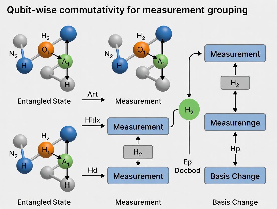
Figure 1: Measurement workflow using Qubit-Wise Commutativity (QWC) grouping.

Full Commutativity (FC)

Definition: Two Pauli strings ( P ) and ( Q ) fully commute if their commutator ( [P, Q] = PQ - QP = 0 ), regardless of whether they commute qubit-wise.

Implications for Measurement: FC is a weaker condition than QWC, allowing for larger and fewer groups. Measuring a fully commuting group requires a unitary ( \hat{U}_{\alpha} ) that can be a multi-qubit Clifford circuit. While this can be compiled efficiently, it results in a deeper circuit than the single-qubit rotations used for QWC groups [19]. This introduces a trade-off: reduced measurement count at the cost of increased circuit depth and potential gate errors.

k-Commutativity: An Interpolating Framework

Definition: A recently introduced framework, k-commutativity, interpolates between QWC ((k=1)) and FC ((k=n)). Two Pauli strings are defined to k-commute if the string can be divided into contiguous blocks of size (k), and the corresponding blocks of the two Paulis commute [21].

Implications for Measurement: This framework provides a smooth trade-off. Grouping by (k)-commutativity allows for a reduced number of groups compared to QWC, while the required unitary ( \hat{U}_{\alpha} ) is less complex and of lower depth than that for a fully commuting group. As ( k ) increases, the number of groups decreases, but the circuit depth required for the basis transformation increases [21]. This offers a tunable parameter for optimizing measurement protocols based on specific hardware capabilities and error profiles.

Figure 2: Workflow for the k-commutativity grouping framework.

Experimental Protocols and Methodologies

This section details the practical methodologies for implementing the grouping strategies discussed, enabling researchers to replicate and apply these techniques.

Protocol 1: Greedy Grouping with Qubit-Wise Commutativity

This is a widely used heuristic for constructing measurement fragments.

• Objective: To partition the Hamiltonian's Pauli terms into a minimal number of QWC groups.
• Procedure:
  • Input: List of Pauli terms ( {P^{[\alpha]}} ) and their coefficients ( {c^{[\alpha]}} ).
  • Initialize: Create an empty list of groups ( G ).
  • Iterate: While the list of Pauli terms is not empty: a. Select the first term ( P ) in the list as a seed for a new group ( G{\text{new}} ). b. For every remaining term ( Q ) in the list, check if ( Q ) qubit-wise commutes with every term currently in ( G{\text{new}} ). c. If yes, move ( Q ) into ( G{\text{new}} ). d. Add ( G{\text{new}} ) to the list of groups ( G ).
• Considerations: The greedy nature of this algorithm makes it fast and simple to implement. However, the initial ordering of the Pauli terms can influence the final number of groups, and the solution is not guaranteed to be globally optimal. Furthermore, it only utilizes QWC, potentially missing opportunities for larger groups afforded by FC.

Protocol 2: Overlapping Grouping via Covariance Estimation

A more advanced strategy moves beyond disjoint groups, allowing a single Pauli term to be measured in multiple different fragments.

• Objective: Leverage the compatibility of some Pauli terms with multiple groups to create an optimized measurement strategy that minimizes the total estimator variance.
• Procedure:
  • Input: A set of candidate measurable groups ( { \hat{A}{\alpha} } ) (which can be generated via QWC, FC, or other methods).
  • Identify Overlaps: For each Pauli term ( P^{[\alpha]} ), list all groups in which it can be measured.
  • Covariance Estimation: Using a classical proxy (e.g., Hartree-Fock state) or preliminary quantum measurements, estimate the covariance matrix ( \text{Cov}{\psi}(\hat{A}{\alpha}, \hat{A}{\beta}) ) between the fragments.
  • Optimize Measurement Allocation: Solve a convex optimization problem to determine the number of measurements ( m{\alpha} ) to allocate to each fragment ( \hat{A}{\alpha} ), minimizing the total variance ( \text{Var}(\sum{\alpha} w{\alpha} \bar{A}{\alpha}) ) for a linear estimator, subject to ( \sum{\alpha} m_{\alpha} = M ) [19].
• Considerations: This framework is general and can lead to a severalfold reduction in the number of measurements compared to non-overlapping methods [19]. It connects traditional grouping approaches with modern techniques from shadow tomography. The primary overhead is the need for a priori variance or covariance estimates.

Table 2: Comparison of Measurement Grouping Frameworks

Framework	Grouping Condition	Circuit Depth for U_α	Number of Groups	Key Advantage	Key Disadvantage
Qubit-Wise Commutativity (QWC)	Commute on every qubit	Low (Single-qubit gates)	Highest	Minimal circuit depth, low error	Largest number of groups
Full Commutativity (FC)	Commute as operators	High (Multi-qubit Cliffords)	Lowest	Minimal number of groups	Higher circuit depth and gate errors
k-Commutativity	Commute on blocks of k qubits	Medium (Tunable with k)	Medium (Tunable with k)	Provides a smooth trade-off between group count and circuit depth	Requires selection of optimal k
Overlapping Groups	Compatible with multiple groups (QWC/FC/k)	Depends on base groups	Depends on base groups	Can achieve lowest total variance	Requires covariance estimation and optimization

Case Study: High-Precision Measurement on Near-Term Hardware

A 2024 study by Korhonen et al. provides a concrete example of applying advanced measurement techniques to achieve high-precision results relevant to drug development [20].

• System: The Boron-dipyrromethene (BODIPY) molecule, a fluorescent dye used in medical imaging and biolabelling, was studied in active spaces ranging from 8 to 28 qubits.
• Objective: Estimate the energy of the Hartree-Fock state for the ( S0 ), ( S1 ), and ( T_1 ) electronic states to chemical precision (1.6 mHa).
• Techniques Applied:
  • Informationally Complete (IC) Measurements: Allowed for the estimation of multiple observables from the same data and provided a seamless interface for error mitigation.
  • Quantum Detector Tomography (QDT): Characterized and mitigated readout errors.
  • Locally Biased Random Measurements: A shot-frugal technique that prioritizes measurement settings with a larger impact on the energy estimation.
  • Blended Scheduling: Mitigated time-dependent noise by interleaving circuits for different Hamiltonians and QDT.
• Result: The combined techniques reduced the measurement error by an order of magnitude, from 1-5% down to 0.16%, bringing the result close to the target chemical precision despite high native readout errors (~1-2%) [20]. This demonstrates a viable path forward for precise molecular energy estimation on noisy hardware.

The Scientist's Toolkit: Essential Research Reagents

The following table details key computational and methodological "reagents" essential for conducting research in Hamiltonian measurement reduction.

Table 3: Key Research Reagent Solutions for Measurement Grouping Experiments

Reagent / Solution	Function / Purpose	Implementation Notes
Pauli String Grouping Library (e.g., in Qiskit)	Implements algorithms (greedy, graph coloring) to group Pauli terms by QWC, FC, or k-commutativity.	Core utility for any measurement reduction protocol. Often integrated into quantum chemistry SDKs.
Classical Proxy Wavefunction (e.g., Hartree-Fock, CISD)	Provides initial estimates of ( \langle \psi	\hat{A}_{\alpha}	\psi \rangle ) and ( \text{Var}{\psi}(\hat{A}{\alpha}) ) for measurement allocation optimization.	Crucial for overlapping grouping and shot-allocation strategies. Accuracy of the proxy influences efficiency.
Clifford Circuit Compiler	Compiles the unitary ( \hat{U}_{\alpha} ) for rotating a group of commuting operators into the Z-basis into native gates.	Required for FC and k-commutativity grouping. Efficiency of compilation affects final circuit depth.
Quantum Detector Tomography (QDT) Toolbox	Characterizes the noisy readout matrix of the quantum device to build an unbiased estimator for observables.	Essential for high-precision work, as it directly mitigates readout error [20].
Variance/Covariance Estimator	Calculates the covariance matrix ( \text{Cov}{\psi}(\hat{A}{\alpha}, \hat{A}_{\beta}) ) for a given state and set of fragments.	Foundational component for the overlapping grouping framework.
Shot Allocation Optimizer	Solves the convex optimization problem to distribute a fixed number of shots among fragments to minimize total estimator variance.	Turns variance estimates into an actionable measurement plan.
2-C-methyl-D-erythritol 4-phosphate	2-C-methyl-D-erythritol 4-phosphate, CAS:206440-72-4, MF:C5H13O7P, MW:216.13 g/mol	Chemical Reagent
Batatasin Iv	Batatasin Iv, CAS:60347-67-3, MF:C15H16O3, MW:244.28 g/mol	Chemical Reagent

The scaling of molecular Hamiltonians presents a formidable measurement challenge for quantum computing applications in drug development. The number of Pauli terms grows rapidly with system size, necessitating sophisticated strategies to make energy estimation feasible. The framework of qubit-wise commutativity provides a critical foundation for this task, enabling the grouping of terms into simultaneously measurable fragments with low circuit overhead. The development of more advanced concepts, such as k-commutativity and overlapping groups, offers a path to further significant reductions in measurement cost. As demonstrated by experimental implementations on current hardware, the combination of these grouping techniques with robust error mitigation can achieve the high precision required for meaningful molecular simulations. For researchers in the field, mastering these protocols and leveraging the associated "toolkit" of computational reagents is essential for pushing the boundaries of what is possible in quantum-accelerated drug discovery.

In the pursuit of practical quantum computing on Noisy Intermediate-Scale Quantum (NISQ) devices, efficient measurement strategies are paramount. The variational quantum eigensolver (VQE) and the quantum approximate optimization algorithm (QAOA), which are leading algorithms for quantum chemistry and optimization problems, require estimating the expectation value of a Hamiltonian. This Hamiltonian is typically a complex sum of numerous Pauli terms. A naïve approach of measuring each term independently in a separate quantum circuit is prohibitively expensive and wasteful of limited quantum resources.

This technical guide details the core concepts of Pauli Words, Observable Grouping, and Simultaneous Measurement as a unified framework for radically reducing the measurement overhead in quantum algorithms. The process is framed within the critical research context of qubit-wise commutativity (QWC), a specific and practical criterion for measurement grouping. By grouping compatible observables, researchers can measure multiple terms in a single circuit execution, minimizing the number of circuit runs, reducing the impact of noise, and accelerating the path to obtaining meaningful scientific results, such as in computational drug development.

Mathematical Foundations: Pauli Words and Commutativity

Pauli Words and Strings

A Pauli Word (or Pauli String) describes a multi-qubit operator defined as the tensor product of single-qubit Pauli operators. The fundamental Pauli operators are the identity (I) and the three Pauli matrices (X), (Y), and (Z) [22]. A Pauli Word (P) can be written as: [ P = \sigma^{(1)} \otimes \sigma^{(2)} \otimes \cdots \otimes \sigma^{(n)} ] where each (\sigma^{(i)} \in {I, X, Y, Z}) acts on the (i)-th qubit [23].

In software libraries like Cirq and PennyLane, these are implemented as core objects. For example, in PennyLane, a PauliWord is an immutable dictionary that maps wires (qubits) to their respective Pauli operators [23].

Table: Fundamental Single-Qubit Pauli Operators

Operator	Matrix Representation	Eigenvalues	Description
(I)	(\begin{pmatrix} 1 & 0 \ 0 & 1 \end{pmatrix})	(+1)	Identity operator
(X)	(\begin{pmatrix} 0 & 1 \ 1 & 0 \end{pmatrix})	(\pm1)	Bit-flip operator
(Y)	(\begin{pmatrix} 0 & -i \ i & 0 \end{pmatrix})	(\pm1)	Phase-bit-flip operator
(Z)	(\begin{pmatrix} 1 & 0 \ 0 & -1 \end{pmatrix})	(\pm1)	Phase-flip operator

Commutation and Anti-Commutation

The commutativity of Pauli Words is the cornerstone of simultaneous measurement. The commutator of two operators (A) and (B) is defined as ([A, B] = AB - BA). If ([A, B] = 0), the operators commute; otherwise, they do not.

Pauli operators obey specific commutation and anti-commutation relations [22]:

• Commutation Relation: ([\sigmaj, \sigmak] = 2i\varepsilon{jkl}\sigmal)
• Anti-commutation Relation: ({\sigmaj, \sigmak} = 2\delta_{jk}I)

Here, (\varepsilon{jkl}) is the Levi-Civita symbol and (\delta{jk}) is the Kronecker delta. Two Pauli Words commute if the number of qubits on which their corresponding single-qubit Paulis anti-commute is even. If this count is odd, they anti-commute [24].

The Principle of Simultaneous Measurement

Theoretical Basis

In quantum mechanics, two observables can be measured simultaneously if and only if their corresponding operators commute [24]. Commuting operators share a common set of eigenvectors. Measuring one observable in this shared eigenbasis projects the quantum state into a joint eigenvector of all commuting observables in the group, allowing the outcomes for all of them to be determined from the same measurement data without disturbing the state for the others [25].

For example, measuring the two-qubit Pauli observable (Z \otimes Z) is equivalent to measuring the parity of the two qubits. The measurement distinguishes between states where the qubits are the same ((|00\rangle), (|11\rangle), eigenvalue (+1)) and states where they are different ((|01\rangle), (|10\rangle), eigenvalue (-1)) [26]. This single measurement provides information about the correlation between the qubits, which is non-locally stored and not accessible by measuring individual qubits alone [26].

Qubit-Wise Commutativity (QWC)

Full commutativity (([A, B] = 0)) is a strict condition. A more relaxed but highly practical criterion is Qubit-Wise Commutativity (QWC). Two Pauli Words (A) and (B) are said to qubit-wise commute if, for every qubit (i), the single-qubit Pauli operators (\sigma^{(i)}A) and (\sigma^{(i)}B) commute [17].

This means that for each qubit, the corresponding Paulis must be either the same or the identity. Formally, for all (i), ([\sigma^{(i)}A, \sigma^{(i)}B] = 0). For example:

• (X \otimes I) and (Z \otimes I) do not QWC (on the first qubit, (X) and (Z) anti-commute).
• (X \otimes Z) and (X \otimes I) do QWC (same on first qubit, (Z) and (I) commute on the second).

QWC is a stronger condition than general commutativity; all QWC pairs commute, but not all commuting pairs are QWC. Its key advantage is operational simplicity: if observables QWC, they can be measured simultaneously by measuring each qubit individually in a basis determined by its non-identity Pauli operator in the group [17].

Observable Grouping Methodologies and Protocols

The process of observable grouping transforms a Hamiltonian (H = \sumi ci Pi) (where (Pi) are Pauli Words) into a minimal set of groups where all observables within a group can be measured simultaneously.

The Observable Grouping Workflow

The following diagram illustrates the complete workflow for efficient measurement via observable grouping.

Detailed Grouping Protocols

Protocol 1: Greedy Qubit-Wise Commutativity (QWC) Grouping

This is a common and efficient grouping strategy [17].

• Input: A list of Pauli Words ( {P1, P2, ..., P_k} ) from a Hamiltonian.
• Initialization: Create an empty list groups.
• Iteration: For each Pauli Word (Pi) in the list:
  • Check against each existing group in groups.
  • If (Pi) qubit-wise commutes with every observable in an existing group, add (Pi) to that group.
  • If no such group is found, create a new group containing (Piand add it togroups`.
• Output: The list groups, where each group is a set of qubit-wise commuting observables.

Protocol 2: Graph-Theoretic Minimum Clique Cover (MCC)

A more advanced method that can find fewer, larger groups, albeit with higher classical computational cost [17].

• Input: A list of Pauli Words ( {P1, P2, ..., P_k} ).
• Graph Construction: Create a graph (G) where:
  • Each vertex represents a Pauli Word (P_i).
  • An edge connects two vertices (Pi) and (Pj) if they commute (or QWC, depending on the criterion used).
• Clique Cover: Solve the Minimum Clique Cover problem on graph (G`. A clique is a subset of vertices where every two distinct vertices are connected. The clique cover is a set of cliques that covers all vertices.
• Output: Each clique in the cover corresponds to a group of simultaneously measurable observables.

Circuit Construction and Measurement

Once observables are grouped, a single quantum circuit is generated for each group.

• Basis Transformation: For a given group, determine the required single-qubit basis change for each qubit. This is defined by the non-identity Pauli operator(s) acting on that qubit within the group [26]:
  • To measure (Z), no change is needed (measure in computational basis).
  • To measure (X), apply a Hadamard gate (H) before measurement.
  • To measure (Y), apply (S^\dagger) followed by (H) before measurement.
• Execution: Run the transformed circuit on a quantum processor or simulator for a sufficient number of "shots" (repetitions) to gather statistics.
• Post-Processing: From the resulting bitstrings, calculate the expectation value (\langle Pi \rangle) for each Pauli Word in the group. The expectation value of the Hamiltonian is then reconstructed as (\langle H \rangle = \sumi ci \langle Pi \rangle) [17].

Table: Basis Transformations for Pauli Measurement

Target Pauli	Diagonalizing Gate Sequence	Equivalent Q# Operation
(Z)	(I)	Measure([PauliZ], [q])
(X)	(H)	Measure([PauliX], [q])
(Y)	(S^\dagger), then (H)	Measure([PauliY], [q])

Resource Analysis and Performance Gains

The resource savings from observable grouping are substantial and critical for applying VQE to problems in chemistry and drug development, such as determining molecular energies.

Quantitative Performance Data

The table below summarizes the typical reduction in the number of required measurement circuits achieved through different grouping strategies for various problem types [17].

Table: Measurement Grouping Performance for Quantum Algorithms

Application	Problem Instance	No Grouping	Wire Grouping	QWC Grouping	Savings vs. Naïve
QAOA	Max-Cut (QUBO)	~180	~25	~1	~99%
Quantum Chemistry (VQE)	H(_2) Molecule	15	7	5	~67%
Quantum Chemistry (VQE)	LiH Molecule	637	295	122	~81%
Quantum Chemistry (VQE)	H(_6) Molecule	3873	1565	599	~85%

The Researcher's Toolkit: Software and Libraries

Several quantum software libraries provide built-in functionalities to automate observable grouping.

Table: Essential Software Tools for Observable Grouping Research

Tool / Library	Grouping Functionality	Key Feature
PennyLane	qml.grouping.group_observables	Supports both "qwc" and "commuting" (general) grouping strategies directly integrated into its QNode execution pipeline [17].
Qiskit	CircuitSampler with grouping plugins	Offers observable grouping utilities, often through plugins designed for advanced algorithms like VQE [17].
Divi (Qoro)	High-level API abstraction	Automates the entire workflow from grouping to execution and post-processing, leveraging lower-level engines like PennyLane to simplify the user experience [17].
Cirq	PauliString and PauliSum objects	Provides the fundamental data structures for representing and manipulating linear combinations of Pauli terms, which are the prerequisites for implementing grouping algorithms [27].
10-Decarbamoyloxy-9-dehydromitomycin B	Mitomycin H	Research-grade Mitomycin H for laboratory investigation. This product is for Research Use Only (RUO) and not for human or veterinary diagnostic or therapeutic use.
Carteolol	Carteolol Hydrochloride	Carteolol is a non-selective beta-adrenergic antagonist for research applications. This product is For Research Use Only (RUO). Not for human or veterinary use.

Experimental Protocol: Applying QWC to a VQE Simulation

This section provides a detailed, step-by-step protocol for running a VQE simulation with observable grouping, representative of an experiment to compute the ground state energy of a molecule like H(_2).

Step-by-Step Protocol

• Problem Formulation:

  • Input: Choose a molecule (e.g., H(_2)) and an interatomic distance.
  • Action: Use a quantum chemistry package (e.g., OpenFermion, Pennylane's qchem module) to generate the electronic structure Hamiltonian (H) in the Pauli basis. The output will be a list of coefficients (ci) and corresponding Pauli Words (Pi).

• Observable Grouping:

  • Input: The list of ({(ci, Pi)}) from Step 1.
  • Action: Apply the Greedy QWC Grouping protocol (Section 4.2, Protocol 1) to this list. The output is (M) groups, (G1, G2, ..., G_M).

• Ansatz and Parameter Initialization:

  • Input: The number of qubits (n) and a chosen parameterized quantum circuit (ansatz), e.g., the Unitary Coupled Cluster (UCC) ansatz or a hardware-efficient ansatz.
  • Action: Initialize the variational parameters (\vec{\theta}) to a starting guess (e.g., zeros, or a random value).

• Quantum Circuit Execution Loop (For each optimization step):

  • For each group (Gj):
    • Construct the parameterized ansatz circuit with the current parameters (\vec{\theta}).
    • Append Measurement Circuitry: For each qubit, determine the necessary basis-changing gates (see Table in Section 4.3) based on the non-identity Pauli operators in group (Gj.</li> <li>Execute the complete circuit on a quantum backend for (S) shots (e.g., (S = 10,000).
    • Collect the measurement results (bitstrings).
  • Classical Post-Processing:
    • For each Pauli Word (Pi) in group (Gj), estimate its expectation value (\langle Pi \rangle) from the bitstrings obtained from (Gj)'s circuit.
    • Compute the total energy estimate: (E(\vec{\theta}) = \sumi ci \langle P_i \rangle`.

• Classical Optimization:

  • Input: The computed energy (E(\vec{\theta})).
  • Action: Use a classical optimizer (e.g., Nelder-Mead, BFGS) to propose new parameters (\vec{\theta}_{\text{new}}) with the goal of minimizing (E(\vec{\theta})).
  • Loop: Repeat from Step 4 until convergence in energy is achieved.

The following diagram visualizes the iterative quantum-classical loop of the VQE algorithm, highlighting the integration of observable grouping.

Observable grouping, particularly using the qubit-wise commutativity criterion, is not merely an optional optimization but a fundamental technique for enabling practical quantum simulations on near-term hardware. By transforming the measurement problem into a classical problem of graph coloring or clique covering, researchers can achieve order-of-magnitude reductions in the quantum resource requirements for algorithms like VQE and QAOA. As quantum hardware continues to mature, the development of more sophisticated grouping strategies and their seamless integration into high-level quantum software stacks will be crucial for tackling increasingly complex problems in fields such as drug discovery and materials science.

Implementing QWC Grouping: From Theory to Practice in Quantum Chemistry Simulations

Step-by-Step Workflow for Observable Grouping and Measurement

In the Noisy Intermediate-Scale Quantum (NISQ) era, efficiently extracting information from quantum systems represents one of the most significant practical bottlenecks for applications ranging from quantum chemistry to optimization problems. The fundamental challenge stems from the need to measure complex molecular Hamiltonians, which are typically decomposed into sums of Pauli terms. For even modest-sized molecules, this decomposition can yield hundreds or thousands of individual terms requiring measurement. For instance, the water molecule (H₂O) requires measuring 1,086 Hamiltonian terms when mapped to a 14-qubit system [15]. A naïve approach of measuring each term in separate quantum circuits creates prohibitive overhead that scales polynomially with system size, making practical quantum advantage impossible without optimization strategies.

This technical guide addresses this "measurement problem" by providing a comprehensive workflow for observable grouping—a powerful technique that significantly reduces quantum resource requirements. We frame this discussion within ongoing research on qubit-wise commutativity, a specific commutativity relation that enables particularly efficient measurement protocols. By grouping compatible observables that can be measured simultaneously, researchers can reduce measurement overhead by up to 90% in some cases [15], dramatically accelerating variational algorithms like the Variational Quantum Eigensolver (VQE) and Quantum Approximate Optimization Algorithm (QAOA) that are essential for quantum chemistry and drug discovery applications.

Theoretical Foundations: From Commutativity to Practical Grouping

Pauli Decomposition and the Measurement Problem

Quantum algorithms for electronic structure problems, particularly the Variational Quantum Eigensolver, estimate molecular ground state energies by measuring the expectation value of a qubit Hamiltonian ( H ), expressed as: [ H = \sumi ci hi ] where each ( hi ) is a Pauli string (tensor product of Pauli operators ( I, \sigmax, \sigmay, \sigmaz )) and ( ci ) are real coefficients [15]. The expectation value ( \langle H \rangle ) is obtained by measuring each term separately and computing the weighted sum: [ \langle H \rangle = \sumi ci \langle h_i \rangle ]

The measurement problem arises because each term ( \langle h_i \rangle ) typically requires numerous repetitions ("shots") on quantum hardware to achieve statistical precision, with the number of terms growing rapidly with molecular size. This creates a computational bottleneck, especially when quantum hardware access is limited and expensive [15].

Commutativity Relations for Observable Grouping

Observable grouping exploits the fundamental quantum mechanical property of commutativity to reduce measurement overhead. Two observables can be measured simultaneously if they commute, meaning their measurement order does not affect the outcomes. For Pauli strings, several commutativity relations enable practical grouping:

• Full Commutativity: Two Pauli strings ( P ) and ( Q ) fully commute if ( [P, Q] = PQ - QP = 0 ). Fully commuting observables share a common eigenbasis and can be measured together using an appropriate basis transformation circuit [16].

• Qubit-Wise Commutativity (QWC): Two Pauli strings ( P = \bigotimes{i=1}^n pi ) and ( Q = \bigotimes{i=1}^n qi ) qubit-wise commute if ( [pi, qi] = 0 ) for all qubits ( i ). This stronger condition implies full commutativity but not vice versa [16]. The significance of QWC is that it enables measurement with minimal circuit depth—typically requiring only single-qubit gates to diagonalize the observables simultaneously.

• ( k )-Commutativity: A recently introduced generalization that interpolates between qubit-wise commutativity (( k=1 )) and full commutativity (( k=n )). Two Pauli strings ( k )-commute if they commute when restricted to blocks of size ( k ) [16]. This provides a tunable trade-off between measurement circuit depth and the number of measurement groups.

The mathematical relationship between these commutativity concepts creates a hierarchical structure where qubit-wise commutativity implies ( k )-commutativity for all ( k \geq 1 ), which in turn implies full commutativity.

Algorithmic Framework for Grouping Strategies

The core algorithmic challenge in observable grouping is to partition the set of Hamiltonian Pauli terms into the minimum number of groups where all members within each group satisfy a specific commutativity relation. This can be framed as a graph coloring problem where vertices represent Pauli terms and edges connect commuting observables [17].

Table 1: Comparison of Observable Grouping Strategies

Grouping Strategy	Commutativity Criterion	Circuit Depth	Number of Groups	Best Use Cases
Qubit-Wise Commutativity (QWC)	Commutation on each qubit	Minimal (single layer of single-qubit gates)	Higher than full commutativity	NISQ devices with severe depth limitations
Full Commutativity	Traditional commutator vanishes	Higher (requires entangling gates for diagonalization)	Minimal	Fault-tolerant systems or high-coherence hardware
( k )-Commutativity	Commutation on blocks of size ( k )	Intermediate (depends on ( k ))	Intermediate, tunable	Balanced performance when moderate depth is acceptable
Classical Shadows	Randomized measurements	Varies	Not applicable (different approach)	Measuring many different observables

The following diagram illustrates the conceptual relationship between these grouping strategies and their resource requirements:

Figure 1: Relationship between grouping strategies and their resource trade-offs. Qubit-wise commutativity requires the most groups but minimal circuit depth, while full commutativity requires fewer groups but greater depth. k-commutativity provides a tunable intermediate approach.

Step-by-Step Workflow for Observable Grouping and Measurement

Step 1: Hamiltonian Preparation and Pauli Decomposition

The workflow begins with generating the qubit Hamiltonian for the target molecular system:

• Molecular Specification: Define the molecular structure (atomic species, coordinates, charge, spin multiplicity) and select a basis set (e.g., STO-3G, 6-31G) for electronic structure calculation.

• Qubit Hamiltonian Generation:

  • Perform a classical Hartree-Fock calculation to obtain molecular orbitals
  • Select an active space for correlated calculations if necessary
  • Transform the electronic Hamiltonian to qubit representation using Jordan-Wigner or Bravyi-Kitaev transformation [15]
  • Output the Hamiltonian as a linear combination of Pauli strings: ( H = \sumi ci P_i )

For example, a hydrogen molecule (Hâ‚‚) at bond length 0.7 angstroms yields a 4-qubit Hamiltonian with 15 Pauli terms after Jordan-Wigner transformation [15].

Step 2: Commutativity Analysis and Group Identification

This critical step identifies compatible observables that can be measured together:

• Construct Commutativity Graph: Create a graph where each vertex represents a Pauli term, and edges connect terms satisfying the chosen commutativity relation (QWC, full commutativity, or ( k )-commutativity).

• Graph Coloring Algorithm: Apply a graph coloring algorithm to partition the vertices into the minimum number of groups where all group members are connected (commuting). While exact graph coloring is NP-hard, efficient heuristic algorithms like largest-first or DSatur provide near-optimal solutions for practical problem sizes [17].

• Group Refinement: For large Hamiltonians, consider iterative refinement or specialized algorithms for specific commutativity relations. For QWC, a greedy algorithm that assigns observables to unused qubits is particularly effective [17].

Table 2: Measurement Overhead Reduction Through Grouping for Molecular Systems

Molecule	Qubit Count	Total Pauli Terms	Groups (No Grouping)	Groups (QWC)	Reduction Percentage
Hâ‚‚	4	15	15	8	~47% [15]
LiH	10	437	437	~120	~73% [28]
Hâ‚‚O	14	1,086	1,086	~250	~77% [15]
BeHâ‚‚	14	1,159	1,159	~260	~78% [28]

Step 3: Diagonalizing Circuit Construction

For each measurement group, construct a quantum circuit that simultaneously diagonalizes all observables in the group:

• Qubit-Wise Commutativity Groups: For QWC groups, the diagonalization circuit consists only of single-qubit gates. For each qubit, if the Pauli operators across the group include non-Z operators, apply the appropriate basis rotation:

  • X measurement: Apply H gate
  • Y measurement: Apply S† followed by H gate
  • Z measurement: No gate needed (already in computational basis)

• Full Commutativity Groups: For fully commuting groups that don't satisfy QWC, construct a Clifford circuit ( U ) such that ( UPiU^\dagger ) is a diagonal Pauli string for all ( Pi ) in the group. This can be implemented using ( O(n^2/\log n) ) Clifford gates [16], though more efficient compilations exist for smaller groups.

• ( k )-Commutativity Groups: For ( k )-commuting groups, the diagonalization circuit has a block structure, with each block of size ( k ) diagonalized independently. This typically requires fewer entangling gates than full diagonalization while achieving better group consolidation than QWC.

The following diagram illustrates the circuit construction process for a QWC group:

Figure 2: Quantum circuit construction workflow for a qubit-wise commuting (QWC) group. After state preparation, compatibility analysis identifies simultaneously measurable observables, single-qubit rotations diagonalize the group, and measurement in the computational basis enables classical post-processing to extract individual expectation values.

Step 4: Quantum Execution and Shot Allocation

Execute the measurement circuits on quantum hardware or simulator:

• Circuit Execution: For each measurement group, run the state preparation circuit followed by the diagonalization circuit, then measure in the computational basis.

• Shot Allocation: Distribute the total measurement budget (shots) across groups optimally. Uniform allocation is simple but suboptimal. Variance-based shot allocation assigns more shots to groups with higher estimated variance, significantly reducing the total shots needed for a target precision [28]. For a total shot budget ( N ), allocate to group ( i ) proportionally to ( \frac{|ci|\sigmai}{\sumj |cj|\sigmaj} ), where ( \sigmai ) is the standard deviation of the measurement outcomes for group ( i ).

• Iterative Refinement: For adaptive algorithms like ADAPT-VQE, reuse measurement outcomes from previous iterations when possible. Recent research shows that reusing Pauli measurement results from VQE optimization in subsequent gradient evaluations can reduce average shot usage to 32.29% compared to naïve approaches [28].

Step 5: Classical Post-Processing and Expectation Value Reconstruction

After quantum execution, process the measurement results to extract individual expectation values:

• Result Aggregation: For each measurement group, collect the measurement statistics (counts of each bitstring outcome).

• Expectation Value Calculation: For each Pauli term in the group, compute its expectation value from the measurement statistics. For diagonal Pauli strings, this involves weighting the bitstring probabilities by the corresponding eigenvalues ((\pm 1)).

• Hamiltonian Estimation: Reconstruct the total Hamiltonian expectation value using the linear combination: [ \langle H \rangle = \sumi ci \langle P_i \rangle ] where the sum is over all Pauli terms in the Hamiltonian.

Advanced Optimization Techniques

Integration with Variational Quantum Algorithms

For practical quantum chemistry applications, observable grouping must be integrated into variational algorithms like VQE and ADAPT-VQE:

• Static Grouping: Precompute measurement groups once at algorithm initialization. This works well for fixed Hamiltonians but doesn't adapt to changing circuit structures.

• Dynamic Grouping: For adaptive ansatz constructions like ADAPT-VQE, where the operator pool changes each iteration, implement just-in-time grouping of the commutator terms needed for gradient calculations. Research shows grouping commutators of single Hamiltonian terms with multiple pool operators can result in approximately ( 2N ) or fewer mutually commuting sets [28].

• Measurement Reuse: In ADAPT-VQE, Pauli measurement outcomes obtained during VQE parameter optimization can be reused in the subsequent operator selection step, reducing the shot overhead of gradient measurements by approximately 60-70% [28].

Error Mitigation Considerations

Measurement grouping introduces unique error mitigation opportunities and challenges:

• Correlated Errors: Terms measured together experience correlated readout errors, which can be characterized and mitigated using readout error mitigation techniques like measurement error tomography.

• Group-Aware Error Mitigation: Implement error mitigation strategies that account for the specific measurement basis of each group, such as applying different calibration matrices for different diagonalization circuits.

Table 3: Research Reagent Solutions for Observable Grouping Experiments

Tool/Resource	Function	Implementation Examples
Quantum Software Frameworks	Provide foundation for Hamiltonian processing, circuit construction, and result analysis	PennyLane, Qiskit, Cirq [17] [27]
Grouping Algorithms	Implement commutativity analysis and graph coloring for measurement optimization	PennyLane's group_observables function, Qiskit's CommutingPaulisiGroup [17]
High-Level APIs	Simplify implementation of grouping strategies with minimal code	Divi library (wraps PennyLane and Qiskit functionality) [17]
Quantum Hardware/Simulators	Execute the measurement circuits and return results	QuEra, IBM Quantum, IonQ, PennyLane default.qubit [29] [30]
Molecular Data Libraries	Provide precomputed Hamiltonians for common chemical systems	PennyLane's qchem module, OpenFermion [15]

Observable grouping through qubit-wise commutativity and related techniques represents a critical optimization strategy for making quantum algorithms practically feasible on current and near-term quantum hardware. By systematically implementing the step-by-step workflow outlined in this guide—from Hamiltonian preparation through classical post-processing—researchers can dramatically reduce measurement overhead, in some cases by up to 90% [15]. For drug discovery professionals investigating complex molecular systems, these techniques make the difference between computationally feasible and intractable quantum simulations.

The field continues to advance rapidly, with new approaches like ( k )-commutativity [16] and measurement reuse in ADAPT-VQE [28] pushing the boundaries of what's possible with limited quantum resources. As quantum hardware continues to improve in scale and stability—with recent demonstrations of 3,000-qubit systems capable of continuous operation [30]—efficient measurement strategies will remain essential for extracting maximum utility from every quantum circuit execution.

This technical guide provides a comprehensive examination of measurement grouping techniques within PennyLane, focusing specifically on the implementation and practical application of grouping_type parameters. Framed within broader research on qubit-wise commutativity for measurement optimization, this work addresses the critical challenge of measurement overhead in variational quantum algorithms—a significant bottleneck in near-term quantum applications, particularly in quantum chemistry and drug development. By leveraging PennyLane's specialized grouping functionality, researchers can achieve up to 90% reduction in required measurements [15], dramatically improving computational efficiency on noisy intermediate-scale quantum (NISQ) devices. This guide presents detailed methodologies, quantitative comparisons, and practical implementation protocols to enable researchers to effectively integrate these optimization strategies into their quantum computing workflows.

In variational quantum algorithms such as the Variational Quantum Eigensolver (VQE), the calculation of expectation values for molecular Hamiltonians represents a fundamental computational bottleneck. The standard approach requires measuring each Pauli term individually, leading to exponentially growing resource requirements as molecular size increases. For example, while a simple Hâ‚‚ molecule Hamiltonian contains only 15 terms, the water molecule (Hâ‚‚O) requires measuring 1,086 distinct terms [15]. This scaling phenomenon creates impractical resource demands when deploying algorithms on real quantum hardware where measurement access is constrained and costly.

Measurement grouping strategies address this challenge by exploiting the mathematical properties of Pauli operators. Specifically, when observables commute (or qubit-wise commute), they share common eigenbases and can be measured simultaneously in appropriately rotated frames. PennyLane implements this theoretical foundation through sophisticated graph-coloring algorithms that identify compatible observable groupings, dramatically reducing the total number of required quantum circuit executions.

Theoretical Foundations: Commutativity Relations

Mathematical Framework

The core mathematical principle underlying measurement grouping involves commutativity between quantum operators. Two observables A and B are considered compatible if their commutator [A, B] = AB - BA = 0, indicating they share a common set of eigenvectors and can be simultaneously measured [17]. PennyLane's grouping functionality extends this fundamental concept through two primary relational frameworks:

• Qubit-wise Commutativity (QWC): Two Pauli words are qubit-wise commuting if they commute on each qubit individually. Formally, Pauli words P and Q qubit-wise commute if for every qubit i, the single-qubit Pauli operators Páµ¢ and Qáµ¢ commute (i.e., Páµ¢Qáµ¢ = Qáµ¢Páµ¢) [31]. This relation is less strict than full commutativity, allowing for larger measurement groups.

• Full Commutativity (FC): Two Pauli words fully commute if their total commutator [P, Q] = 0, without the qubit-wise restriction. This stricter condition typically results in more, smaller measurement groups but may be necessary for certain computational frameworks [12].

The GALIC framework proposes a hybrid approach that interpolates between QWC and FC relations, demonstrating a 20% reduction in estimator variance compared to standard QWC grouping while maintaining accuracy in Hamiltonian estimation [12].

Graph-Theoretic Implementation

PennyLane formulates the grouping problem using graph theory, where each Pauli word becomes a vertex in a graph, and edges represent the failure of the chosen commutativity relation [31]. Grouping compatible observables then reduces to finding the minimum clique cover problem, which is equivalent to graph coloring on the complementary graph. Since both problems are NP-hard, PennyLane employs heuristic graph coloring algorithms:

• Largest First (lf): Orders nodes by degree before coloring
• Recursive Largest First (rlf): Recursively identifies large independent sets
• Degree of Saturation (dsatur): Prioritizes nodes with the most used colors among neighbors
• Independent Set (gis): Builds color classes around maximal independent sets [31]

PennyLane Grouping Implementation

Core Grouping Functions

PennyLane provides multiple access points for measurement optimization, each designed for specific use cases and computational requirements:

Table 1: PennyLane Measurement Grouping Functions

Function	Primary Use Case	Key Parameters	Output
PauliGroupingStrategy	Low-level grouping control	grouping_type, graph_colourer	Grouped observables
optimize_measurements	High-level measurement optimization	grouping, colouring_method	Rotations, groupings, coefficients
split_non_commuting	Circuit transformation	grouping_strategy, shot_dist	Multiple executable tapes

PauliGroupingStrategy Class

The PauliGroupingStrategy class provides the foundational infrastructure for observable partitioning in PennyLane. As implemented in the source code, this class "partition[s] a list of Pauli words according to some binary symmetric relation" by formulating the list as a graph where "nodes represent Pauli words and edges between nodes denotes that the two corresponding Pauli words satisfy the symmetric binary relation" [31].

Initialization Parameters:

• observables: List of Pauli words to partition
• grouping_type: Binary relation defining partitions ('qwc', 'commuting', 'anticommuting')
• graph_colourer: Heuristic coloring algorithm ('lf', 'rlf', 'dsatur', 'gis')

The class employs cached properties for computational efficiency, including binary_observables (symplectic representation) and adj_matrix (complement graph adjacency) [31].

optimize_measurements Function

The optimize_measurements function provides a higher-level interface that "partitions then diagonalizes a list of Pauli words, facilitating simultaneous measurement of all observables within a partition" [32]. This function combines grouping with the practical generation of diagonalizing rotations, returning executable measurement protocols.

Example Implementation:

This example produces a QWC-optimized measurement scheme where the first group contains Z(0) @ Z(1) and the second contains Z(0) and Z(1), with corresponding diagonalizing rotations [32].

splitnoncommuting Transform

The split_non_commuting transform operates at the circuit level, automatically "splitting a circuit into tapes measuring groups of commuting observables" [33]. This approach integrates seamlessly with PennyLane's QNode architecture, requiring minimal code modification while providing flexible grouping strategies and shot distribution options.

Key Features:

• Multiple grouping strategies ("default", "qwc", "wires", None)
• Configurable shot distribution ("uniform", "weighted", "weighted_random", custom)
• Preservation of measurement ordering in output

Grouping Type Parameterization

The grouping_type parameter fundamentally controls how observables are grouped for simultaneous measurement:

• qwc (Qubit-wise Commuting): The default and typically most efficient method, identifying observables that commute qubit-by-qubit. This approach generally produces the fewest measurement groups but requires the specific condition that "for every qubit i, the single-qubit Pauli operators Páµ¢ and Qáµ¢ commute" [31].

• commuting (Fully Commuting): A stricter grouping that requires full commutativity between all observables in a group. While producing more groups than QWC, this approach may be necessary for certain algorithmic requirements or when specific measurement bases are preferred.

• anticommuting: A specialized grouping strategy that groups anticommuting observables, useful for specific algorithmic applications beyond standard expectation value estimation.

Computational Methodology and Workflow

Experimental Protocol for Measurement Grouping

Implementing effective measurement grouping requires a systematic approach to Hamiltonian preparation, grouping execution, and result analysis:

Step 1: Hamiltonian Generation

• Obtain molecular Hamiltonian through quantum chemistry packages (e.g., PySCF)
• Apply fermion-to-qubit transformation (Jordan-Wigner or Bravyi-Kitaev)
• Extract Pauli terms and coefficients

Step 2: Grouping Strategy Selection

• Evaluate molecular size and qubit count
• Assess classical computational resources for grouping overhead
• Select appropriate grouping_type based on accuracy requirements
• Choose graph coloring heuristic based on Hamiltonian complexity

Step 3: Grouping Execution

• Instantiate grouping class or call optimization function
• Extract measurement groups and diagonalizing rotations
• Validate group commutativity relations

Step 4: Circuit Execution and Analysis

• Execute rotated measurement circuits on target device
• Aggregate results according to grouping structure
• Compare resource usage against ungrouped approach

The Scientist's Toolkit: Essential Research Components

Table 2: Critical Components for Measurement Grouping Research

Component	Function	Implementation Example
Molecular Hamiltonians	Problem specification	qml.data.load('qchem', molname="H2", bondlength=0.7)
Grouping Strategies	Define commutativity relations	grouping_type='qwc' or 'commuting'
Graph Coloring Algorithms	Solve grouping combinatorics	colouring_method='rlf' or 'dsatur'
Diagonalizing Rotations	Enable simultaneous measurement	qml.RY(-1.5707963267948966, wires=[0])
Shot Distribution	Optimize finite-shot allocation	shot_dist='weighted' for coefficient-aware sampling
Diclobutrazol	Diclobutrazol, CAS:66345-62-8, MF:C15H19Cl2N3O, MW:328.2 g/mol	Chemical Reagent
Apricitabine	Apricitabine, CAS:143338-12-9, MF:C8H11N3O3S, MW:229.26 g/mol	Chemical Reagent

Performance Analysis and Benchmarking

Quantitative Efficiency Gains

Measurement grouping strategies demonstrate substantial improvements in computational efficiency across various molecular systems and problem sizes:

Table 3: Measurement Grouping Performance Across Molecular Systems

Molecule	Qubits	Original Terms	QWC Groups	Reduction	Classical Overhead
Hâ‚‚	4	15	2-4	73-87%	Minimal
LiH	12	630	~85	~86%	Moderate
Hâ‚‚O	14	1,086	~150	~86%	Significant
Complex Molecules	20+	10,000+	1,000-1,500	85-90%	Substantial

Data synthesized from performance reports [15] [17] demonstrates consistent measurement reduction of 85-90% across various molecular systems when employing QWC grouping strategies. The Hâ‚‚ molecule shows particularly dramatic improvements, with measurement requirements reduced from 15 terms to as few as 2-4 groups [15] [17].

Algorithmic Overhead Considerations

While measurement grouping provides significant reductions in quantum resource requirements, researchers must consider the classical computational overhead introduced by the grouping process itself. The graph coloring algorithms employed have polynomial complexity, becoming non-trivial for large Hamiltonians with thousands of terms. As system size increases, the selection of graph coloring heuristic impacts both grouping quality and classical computation time:

• rlf (Recursive Largest First): Typically produces the fewest groups but has higher computational complexity
• lf (Largest First): Faster execution with slightly more groups
• dsatur and gis: Intermediate performance characteristics [31]

For large-scale problems, the wires grouping strategy provides a computationally cheaper alternative to QWC, though with potentially less optimal grouping efficiency [33].

Advanced Applications and Future Directions

Quantum Machine Learning Integration

Measurement optimization techniques extend beyond quantum chemistry into quantum machine learning (QML) applications. When training parameterized quantum circuits for classification tasks, efficient measurement strategies reduce the resource requirements for gradient calculations and inference. The integration of grouping methods with hybrid quantum-classical models represents an emerging research frontier with significant practical implications [34].

Device-Aware Grouping Strategies

Recent research, including the GALIC framework, demonstrates that incorporating device-specific characteristics—such as qubit connectivity and noise profiles—into grouping strategies can further enhance performance on NISQ devices. By optimizing for both commutativity relations and hardware constraints, these approaches achieve an additional 20% reduction in estimator variance compared to standard QWC grouping [12].

Shot Allocation Optimization

The split_non_commuting transform's shot_dist parameter enables sophisticated shot allocation strategies across measurement groups. By distributing shots according to coefficient magnitudes ("weighted"), researchers can minimize the overall estimator variance within fixed total shot budgets. For Hamiltonian H = Σcáµ¢Oáµ¢ with grouped terms, optimal shot allocation follows:

[ \text{Shots}k \propto \left| \sum{i \in Gk} ci \right| ]

where Gâ‚– represents the k-th measurement group [33]. This approach typically provides a 10-30% reduction in estimation error compared to uniform shot distribution.

Measurement grouping through PennyLane's grouping_type parameters represents a critical optimization strategy for enabling practical quantum computations on current hardware. By reducing measurement requirements by 85-90% while maintaining mathematical rigor, these techniques directly address one of the most significant bottlenecks in variational quantum algorithms. The continued development of hybrid grouping approaches, device-aware optimization, and sophisticated shot management promises further enhancements to quantum computational efficiency, accelerating progress toward practical quantum advantage in drug development and materials discovery.

The Variational Quantum Eigensolver (VQE) has emerged as a leading algorithm for near-term quantum computers, particularly for solving electronic structure problems in quantum chemistry [15]. A fundamental challenge in scaling VQE beyond classically tractable systems is the "measurement problem"—the exponentially growing number of measurements required to estimate molecular energies accurately [15]. The molecular Hamiltonian, when mapped to qubits via transformations such as Jordan-Wigner or Bravyi-Kitaev, becomes a linear combination of Pauli words:

[ \hat{H} = \sum{i} ci hi, \quad hi = \bigotimes{n=0}^{N-1} Pn ]

where ( Pn \in {I, \sigmax, \sigmay, \sigmaz} ) [15]. Estimating the expectation value ( \langle \psi(\theta) | \hat{H} | \psi(\theta) \rangle ) requires measuring each term ( h_i ), creating a significant bottleneck on quantum hardware [15] [19].

This case study explores the application of Qubit-Wise Commutativity (QWC), a key measurement grouping strategy, to the molecular Hamiltonians of Hâ‚‚ and Hâ‚‚O. We demonstrate how QWC can dramatically reduce the number of measurements required, providing a crucial optimization for practical quantum computational chemistry. Our analysis is framed within broader research efforts to develop efficient measurement protocols for variational quantum algorithms.

Theoretical Foundation: QWC and Measurement Grouping

Commutativity Relations for Measurement Grouping

Two primary commutativity relations enable simultaneous measurement of Pauli terms:

• Full Commutativity (FC): Two Pauli terms ( \hat{P}i ) and ( \hat{P}j ) are fully commuting if ( [\hat{P}i, \hat{P}j] = 0 ). FC groups can be measured simultaneously but may require multi-qubit Clifford gates for diagonalization [19].
• Qubit-Wise Commutativity (QWC): Two Pauli terms ( \hat{P}i ) and ( \hat{P}j ) qubit-wise commute if, for every qubit ( k ), the single-qubit operators ( \hat{\sigma}{i,k} ) and ( \hat{\sigma}{j,k} ) commute [35] [19]. This is a stricter condition than FC, but offers a practical advantage: QWC groups can be diagonalized using only single-qubit Clifford gates [19].

The following diagram illustrates the workflow for grouping and measuring Hamiltonian terms using the QWC strategy:

The GALIC Framework: Extending Beyond Basic QWC

Recent research has developed hybrid approaches that interpolate between FC and QWC. The GALIC (Generalized backend-Aware pauLI Commutation) framework introduces context-aware hybrid FC/QWC commutativity relations that are noise-and-connectivity aware [35]. GALIC maintains estimator accuracy while lowering variance by an average of 20% compared to QWC, demonstrating that advanced grouping strategies can yield significant improvements over basic QWC [35].

QWC Applied to Hâ‚‚ Molecular Hamiltonian

Hâ‚‚ Hamiltonian Structure

For the Hydrogen molecule (Hâ‚‚) at bond length 0.7 Ã…, the qubit Hamiltonian requires 4 qubits and contains 15 Pauli terms [15]:

QWC Grouping Strategy for Hâ‚‚

The Hâ‚‚ Hamiltonian contains terms that can be organized into QWC groups based on their Pauli operators. A practical grouping strategy identifies terms that share compatible measurement bases:

Table: QWC Groups for Hâ‚‚ Hamiltonian

Group	Pauli Terms	Count	Measurement Basis
Group 1	Z(0), Z(1), Z(0) @ Z(1), Z(2), Z(0) @ Z(2), Z(3), Z(0) @ Z(3), Z(1) @ Z(2), Z(1) @ Z(3), Z(2) @ Z(3)	10	Computational (Z) basis
Group 2	Y(0) @ X(1) @ X(2) @ Y(3), Y(0) @ Y(1) @ X(2) @ X(3), X(0) @ X(1) @ Y(2) @ Y(3), X(0) @ Y(1) @ Y(2) @ X(3)	4	Requires basis rotation

Measurement Reduction Analysis

For Hâ‚‚, the naive approach requires 15 separate measurements (one per Pauli term). Using QWC grouping, this can be reduced to significantly fewer measurement settings. In practice, implementing this with PennyLane demonstrates that the number of quantum executions can be optimized to 8 through additional circuit optimizations [15]. This represents a approximately 47% reduction in required measurements.

QWC Applied to Hâ‚‚O Molecular Hamiltonian

Hâ‚‚O Hamiltonian Structure

The water molecule (Hâ‚‚O) presents a more complex computational challenge. Its Hamiltonian requires 14 qubits and contains 1,086 Pauli terms [15]. This exponential growth in term count highlights the critical importance of measurement optimization for practical quantum chemistry applications.

A sample of the Hâ‚‚O Hamiltonian structure shows complex multi-qubit Pauli terms:

The molecular orbital structure of Hâ‚‚O involves 7 basis functions (oxygen 1s, 2s, 2px, 2py, 2pz orbitals and two hydrogen 1s orbitals), leading to the complex Hamiltonian structure when mapped to qubits [36].

QWC Grouping Strategy for Hâ‚‚O

For larger molecules like Hâ‚‚O, systematic grouping algorithms are essential. The greedy coloring approach provides an effective method for QWC grouping:

• Construct QWC Graph: Create a graph where vertices represent Pauli terms and edges connect QWC-compatible terms
• Color the Graph: Assign "colors" (measurement groups) such that no adjacent vertices share the same color
• Minimize Colors: Use greedy algorithms to minimize the number of colors (measurement groups) needed

Table: Measurement Grouping Efficiency for Molecular Hamiltonians

Molecule	Qubits	Pauli Terms	Naive Measurements	QWC Groups	Reduction Rate
Hâ‚‚	4	15	15	~8	~47%
Hâ‚‚O	14	1,086	1,086	Highly optimized grouping can reduce measurements by up to 90% for some systems [15]

Experimental Protocol and Implementation

Research Reagent Solutions

Table: Essential Computational Tools for QWC Experiments

Tool Category	Specific Solution	Function in QWC Experiment
Quantum SDKs	PennyLane [15]	Constructs variational circuits, implements QWC grouping, manages quantum execution
Quantum Chemistry	OpenFermion [15]	Generates molecular Hamiltonians in qubit representation
Grouping Algorithms	Greedy Grouping [19]	Groups commuting Pauli terms to minimize measurement settings
Classical Optimizers	JAX [15]	Provides classical optimization for VQE parameters

Step-by-Step QWC Measurement Protocol

• Hamiltonian Generation

  • Obtain molecular geometry (e.g., Hâ‚‚ bond length: 0.7 Ã…, Hâ‚‚O bond angle: 104.5° [36])
  • Compute electronic Hamiltonian using Hartree-Fock method
  • Apply fermion-to-qubit transformation (Jordan-Wigner or Bravyi-Kitaev)

• QWC Grouping Implementation

  • Extract all Pauli terms and coefficients from the Hamiltonian
  • Build compatibility graph based on QWC relation
  • Apply greedy graph coloring algorithm to form measurement groups

• Quantum Circuit Execution

  • For each QWC group, construct appropriate single-qubit rotation circuits
  • Execute rotated circuits on quantum device or simulator
  • Measure in computational basis and collect statistics

• Energy Estimation

  • Compute expectation values for each Pauli term within groups
  • Calculate total energy as weighted sum: ( E = \sumi ci \langle \psi | h_i | \psi \rangle )

The following diagram illustrates the complete experimental workflow from molecule specification to energy estimation:

Results and Discussion

Performance Analysis of QWC Grouping

Application of QWC grouping to molecular Hamiltonians demonstrates substantial measurement reduction:

• Theoretical Efficiency: QWC grouping can reduce the number of measurements by up to 90% for some systems compared to naive measurement [15]
• Practical Considerations: While QWC provides significant improvements, recent research shows that overlapping grouping methods and hybrid approaches like GALIC can achieve further enhancements [35] [19]
• Variance Implications: The optimal measurement strategy must consider not just the number of groups, but also the variance of estimators within each group [19]

Comparison with Alternative Grouping Strategies

QWC occupies a middle ground in the spectrum of measurement grouping strategies:

• Advantages of QWC:

  • Requires only single-qubit gates for diagonalization
  • Simpler circuit implementation than FC grouping
  • Substantial measurement reduction over naive approaches

• Limitations of QWC:

  • Produces more groups than FC due to stricter commutativity condition
  • May yield higher estimator variance compared to more advanced hybrid methods
  • Does not exploit full Hamiltonian structure like fermionic grouping

Implications for Quantum Computational Chemistry

The application of QWC to molecular systems like Hâ‚‚ and Hâ‚‚O demonstrates that measurement optimization is essential for practical quantum computational chemistry. As molecular size increases, the polynomial reduction in measurements provided by QWC and related techniques becomes crucial for achieving quantum advantage [15]. These developments are particularly relevant for drug development professionals seeking to apply quantum computing to molecular design and optimization.

Qubit-Wise Commutativity provides an effective strategy for reducing quantum measurement overhead in variational quantum algorithms for quantum chemistry. Our case study demonstrates successful application to Hâ‚‚ and Hâ‚‚O molecular Hamiltonians, with measurement reductions up to 90% achievable for some systems. While QWC offers practical advantages through simple circuit implementations, ongoing research into hybrid approaches like GALIC promises further improvements. As quantum hardware continues to evolve, measurement optimization strategies like QWC will play an increasingly vital role in enabling practical quantum computational chemistry applications, including pharmaceutical drug development.

The efficient extraction of information from quantum systems represents a significant challenge in the noisy intermediate-scale quantum (NISQ) era. Quantum algorithms, such as the Variational Quantum Eigensolver (VQE), require measuring complex observables like molecular electronic Hamiltonians, which are typically expressed as sums of numerous Pauli terms [19]. A naive approach of measuring each term independently would consume prohibitive quantum resources, making optimization crucial. This challenge is addressed by framing the measurement optimization problem in terms of fundamental graph algorithms, specifically graph coloring and the minimum clique cover (MCC), which group compatible operators for simultaneous measurement [37] [17].

The core principle relies on the commutativity of operators. Two observables are compatible if they commute, meaning their measurement order does not affect the outcome, allowing them to be measured simultaneously in a shared eigenbasis [17]. In practical terms for quantum computing, this involves identifying Pauli terms that commute (either through full commutativity or the stricter qubit-wise commutativity) and grouping them together. The resulting reduction in the number of distinct measurement circuits directly decreases the required quantum runtime and mitigates the impact of noise on current hardware [19] [17].

This technical guide explores the theoretical foundations and practical applications of graph coloring and minimum clique cover algorithms within this context. We will detail how the grouping problem is mapped to a graph representation, analyze the computational complexity of solving it, and provide experimental protocols and results demonstrating significant performance gains in quantum chemistry simulations.

Graph-Theoretic Foundations and Definitions

Key Graph Concepts

The problem of grouping commuting observables is naturally represented using graph theory. The core concepts are:

• Commutativity Graph (G): An undirected graph G = (V, E) where each vertex in V represents a single Pauli term from the Hamiltonian. An edge (u, v) ∈ E exists between two vertices u and v if and only if their corresponding Pauli terms do not commute [37] [19]. The lack of an edge indicates commutativity.
• Complement Graph (GÌ„): The complement of graph G, denoted GÌ„, has the same vertex set V, but an edge (u, v) exists in GÌ„ if and only if it is not present in G [38] [39]. Therefore, in GÌ„, an edge connects two vertices if their corresponding Pauli terms commute.
• Clique: A subset of vertices C ⊆ V where every two distinct vertices in C are adjacent. In GÌ„, a clique represents a set of mutually commuting Pauli terms [37] [39].
• Independent Set: A subset of vertices where no two are adjacent. In the original commutativity graph G, an independent set represents a set of mutually commuting terms [39].

Formal Problem Definitions

The grouping task can be defined as two equivalent graph problems:

• Minimum Clique Cover (MCC) on GÌ„: A clique cover is a set of cliques C = {C₁, ..., Cₖ} in GÌ„ such that every vertex v ∈ V is contained in at least one clique. The Minimum Clique Cover problem seeks the smallest such k, known as the clique cover number, θ(Ḡ) [37] [39]. Each clique in this cover corresponds to a group of mutually commuting observables that can be measured simultaneously.

• Graph Coloring on G: A graph coloring assigns colors to vertices such that no two adjacent vertices share the same color. The chromatic number, χ(G), is the minimum number of colors required [38]. In our context, a color corresponds to a distinct measurement group, and the adjacency condition in G (non-commutativity) ensures that non-commuting operators are placed in different groups.

A fundamental equivalence connects these two problems: the minimum number of cliques needed to cover GÌ„ is equal to the chromatic number of G, that is, θ(Ḡ) = χ(G) [38] [39]. This duality allows one to choose the more tractable formulation for a given instance, often leveraging well-researched graph coloring heuristics on G to solve the MCC problem on GÌ„.

Figure 1: The logical workflow for mapping a quantum measurement problem onto the dual graph problems of Minimum Clique Cover and Graph Coloring, which are mathematically equivalent.

The Minimum Clique Cover (MCC) Method

Formal Definition and Complexity

The Minimum Clique Cover (MCC) is a fundamental combinatorial optimization problem. For a graph GÌ„ = (V, E), a clique cover is a collection of cliques C = {C₁, ..., Cₖ} where the union of their vertex sets is V. The minimum clique cover number θ(Ḡ) is the smallest such k [37] [39].

The general MCC decision problem is NP-hard, making finding the exact minimum cover computationally intractable for large graphs [37]. This complexity extends to its application in quantum measurement, where the decision variant of determining if a clique cover of size ≤ k exists is NP-complete [37]. Consequently, research has focused on parameterized algorithms for specific graph classes and practical heuristic methods.

Algorithmic Approaches and Bounds

Significant progress has been made in developing efficient algorithms for MCC under certain constraints:

• Parameterized Algorithms: For graphs with bounded degeneracy (d) or clique-number (β), fixed-parameter tractable (FPT) algorithms exist. For example, the ECC-S algorithm for edge clique cover runs in time O*(3^((d+1)k/3)), while the ECC-S2 algorithm achieves O*(2^(8k log k) n^(O(1))) under clique-number parameterization, offering exponential improvements for sparse graphs [37].
• Specialized Graph Classes: In specific graph families, MCC becomes tractable. For (bull, Câ‚„)-free graphs, an exact algorithm with O(n⁴) time complexity exists, leveraging decomposition theorems and combinatorial reductions like removing dominated vertices and using maximum matching in triangle-free subgraphs [37].
• Extremal Bounds: Closed-form upper bounds Θₙ(m) exist for the MCC size in graphs with n vertices and m edges. For sparse graphs (0 ≤ m ≤ ⌊n²/4⌋), the bound is Θₙ(m) = m + n - 2⌊√m⌋ - δ(m), where δ(m) ∈ {0,1}. For denser graphs, the bound involves the number of missing edges k and is given by Θₙ(m) = k + t, where t is the largest integer satisfying t² - t ≤ k [37] [39]. These bounds help gauge the potential improvement from grouping.

Table 1: Algorithmic Results for Minimum Clique Cover and Related Problems

Graph Class / Parameterization	Complexity / Bound	Key Reference
General Graphs (Unparameterized)	NP-hard	(Verteletskyi et al., 2019) [37]
Degeneracy-parameterized (ECC-S)	O*(3^((d+1)k/3))	(Ullah, 2022) [37]
Clique-number-parameterized (ECC-S2)	O*(2^(8k log k) n^(O(1)))	(Ullah, 2022) [37]
(bull, C₄)-free Graphs	O(n⁴) exact algorithm	(Cameron et al., 2017) [37]
Rectangle Intersection (Greedy GCC)	≤ 3√n (empirical bound)	(Mandal et al., 2012) [37]

Graph Coloring for Measurement Grouping

Heuristic Coloring Algorithms

Given the NP-hard nature of optimal graph coloring, heuristic algorithms are employed in practice to find good, though not necessarily minimal, colorings. These heuristics are applied to the commutativity graph G to find measurement groups. Common strategies include [37]:

• Largest First (LF): Orders vertices by descending degree and colors them sequentially.
• Smallest Last (SL): Iteratively removes the vertex with the smallest degree, colors the graph, and then reinserts vertices in reverse order.
• DSATUR: A dynamic saturation degree algorithm that selects the vertex with the most constraints (the highest number of differently colored neighbors) for coloring next.
• Recursive Largest First (RLF): Partitions the graph recursively into colored and uncolored sets, aiming to maximize the size of each color class.

These greedy coloring heuristics run in polynomial time and provide effective groupings for quantum Hamiltonians, often achieving a 3–5× reduction in the number of measurement circuits for small molecules like H₂, LiH, and H₂O [37].

Qubit-Wise Commutativity (QWC) vs. Full Commutativity (FC)

A critical distinction in quantum measurement grouping is the type of commutativity required:

• Qubit-Wise Commutativity (QWC): Two Pauli products commute in a qubit-wise manner if their corresponding single-qubit operators commute on every qubit [19]. This is a stricter condition than full commutativity. The unitary transformation U_α required to diagonalize a QWC group for measurement consists only of single-qubit Clifford gates (e.g., Hadamard gates for X to Z rotation) [19] [17].
• Full Commutativity (FC): Two Pauli products commute if their overall commutator is zero. This allows for larger, more efficient groups but requires more complex diagonalization circuits. The unitary U_α for an FC group may require multi-qubit Clifford gates (e.g., CNOT gates) to transform the group into a tensor product of Z operators [19].

While FC grouping can lead to fewer measurement groups, the increased circuit depth and complexity of the non-local transformations can negate some of the benefits on noisy hardware, making QWC a more practical choice in many NISQ applications [19].

Experimental Protocols and Performance Analysis

Methodology for Quantum Measurement Grouping

The standard experimental protocol for evaluating grouping algorithms in quantum computing involves several well-defined steps [19]:

• Hamiltonian Generation: Generate the qubit Hamiltonian for a target molecule (e.g., Hâ‚‚, LiH, Hâ‚‚O) using a fermion-to-qubit mapping (such as Jordan-Wigner, Bravyi-Kitaev, or parity mapping). This yields a list of Pauli terms P_n and their coefficients c_n.
• Graph Construction: Construct the commutativity graph G. For each pair of Pauli terms, check for commutativity (either QWC or FC). If they do not commute, add an edge between their corresponding vertices in G. The time complexity for building this graph is O(M² N), where M is the number of Pauli terms and N is the number of qubits [37].
• Grouping via Coloring or MCC:
  • Apply a graph coloring heuristic (e.g., DSATUR, RLF) directly to G. Each color class corresponds to a measurement group.
  • Alternatively, construct the complement graph GÌ„ and apply an MCC heuristic (e.g., greedy clique removal). Each clique in the cover is a measurement group.
• Circuit Generation and Execution: For each measurement group, determine the diagonalizing unitary U_α (single-qubit for QWC, potentially multi-qubit for FC). Prepare the trial wavefunction |ψ(θ)⟩, apply U_α, and measure in the standard Z-basis.
• Post-Processing and Estimation: Use the measurement results (bitstrings) to compute the expectation values for each Pauli term in the group. Combine the results across all groups, weighted by their coefficients, to estimate the total energy expectation value ⟨H⟩.

Figure 2: The detailed workflow for a quantum measurement grouping experiment, from Hamiltonian generation to energy estimation.

Quantitative Performance Results

Empirical studies on model molecules consistently demonstrate the significant resource reductions achieved by grouping algorithms. The table below summarizes typical results from the literature, comparing the number of measurement groups required for different molecules and grouping strategies.

Table 2: Measurement Grouping Performance for Molecular Hamiltonians

Molecule (Qubit Mapping)	Total Pauli Terms (M)	Groups (QWC)	Groups (FC)	Reduction Factor	Key Reference
H₂ (BK)	15	3	-	5.0×	(Verteletskyi et al., 2019) [37]
LiH (Parity)	100	25	-	4.0×	(Verteletskyi et al., 2019) [37]
H₂O (BK)	165	34	-	~4.9×	(Verteletskyi et al., 2019) [37]
H₆	-	-	-	3–5× (Typical)	(Izmaylov et al., 2023) [19]
Benchmark Set (VQE)	-	-	-	Severalfold	(Izmaylov et al., 2023) [19]

The "reduction factor" is calculated as M / (# of Groups). These results show that grouping strategies consistently reduce the number of distinct measurements by a factor of 3 to 5 for typical quantum chemistry problems. Furthermore, research indicates that leveraging overlapping fragments—where a Pauli term compatible with multiple groups is assigned to the one that minimizes the overall estimator variance—can achieve a severalfold further reduction in the number of measurements compared to non-overlapping state-of-the-art methods [19].

This section details key software tools and mathematical concepts that form the essential "research reagents" for implementing and experimenting with advanced grouping algorithms.

Table 3: Key Resources for Grouping Algorithm Research

Resource Name / Concept	Type	Primary Function	Relevance to Grouping
PennyLane	Software Library	Hybrid quantum-classical programming	Provides built-in functions (group_observables) for QWC and FC grouping, circuit transformation, and post-processing [40] [17].
Divi	Software Library (High-level API)	Quantum workflow automation	Simplifies grouping by offering a high-level interface that orchestrates PennyLane's lower-level functions, automating the entire measurement pipeline [17].
Qiskit	Software Library	Quantum programming and simulation	Offers plugins and utilities for observable grouping, often within modules related to circuit cutting and error mitigation [17].
Commutativity Graph	Mathematical Model	Abstract representation	The foundational graph model G where vertices are Pauli terms and edges represent non-commutativity [37] [19].
Graph Coloring Heuristic	Algorithm	Approximation algorithm	Practical methods (DSATUR, RLF) for solving the NP-hard coloring problem on G to obtain measurement groups [37].
Clique Cover Number θ(Ḡ)	Graph Invariant	Theoretical bound	The minimum number of groups required; its value or upper bound provides a target for evaluating heuristic performance [37] [39].

Integration with VQE Workflows for Electronic Structure Calculations

The Variational Quantum Eigensolver (VQE) has emerged as a leading algorithm for solving electronic structure problems on near-term quantum computers, but its practical implementation faces significant challenges, particularly regarding measurement efficiency. This technical guide explores the critical role of measurement grouping strategies, with a specific focus on qubit-wise commutativity and its extensions, within VQE workflows for electronic structure calculations. These techniques address a fundamental bottleneck: the exponentially large number of measurements required to estimate the expectation value of molecular and solid-state Hamiltonians. By strategically grouping simultaneously measurable operators, researchers can dramatically reduce the measurement overhead, bringing quantum simulations of complex systems closer to practical reality. This guide provides a comprehensive framework for integrating advanced commutativity-based measurement grouping into VQE workflows, complete with theoretical foundations, practical methodologies, and experimental validation for materials science and drug development applications.

Theoretical Foundations of Measurement Grouping

The Electronic Structure Hamiltonian and Measurement Challenge

In quantum chemistry and materials science, the electronic structure Hamiltonian is typically expressed as a sum of Pauli strings after fermion-to-qubit mapping:

[ H = \sum_{\alpha} c^{[\alpha]} P^{[\alpha]} ]

where each ( P^{[\alpha]} ) is a tensor product of Pauli operators (I, X, Y, Z) and ( c^{[\alpha]} ) is a real coefficient [16]. The VQE algorithm estimates the expectation value ( \langle \psi(\theta) | H | \psi(\theta) \rangle ) by measuring each term in the Hamiltonian. For non-commuting terms, separate measurements are required, leading to a measurement count that can grow exponentially with system size if not properly managed [12].

The Commutativity Spectrum in Measurement Grouping

Measurement grouping strategies exploit commutativity relations between Pauli strings to minimize the number of distinct measurement circuits required. These strategies exist along a spectrum:

• Full Commutativity (FC): Operators that commute can be simultaneously diagonalized by a single Clifford circuit and measured in the same basis [16]. This approach minimizes the number of measurement circuits but requires deeper circuits for basis transformation, with depth scaling as ( O(n^2/\log n) ) for ( n )-qubit systems [16].

• Qubit-Wise Commutativity (QWC): Two Pauli strings ( P = \bigotimes{i=1}^n pi ) and ( Q = \bigotimes{i=1}^n qi ) qubit-wise commute if ( [pi, qi] = 0 ) for all ( i \in [n] ) [16]. QWC groups can be measured with depth-one quantum circuits but typically result in more measurement groups compared to FC.

• ( k )-Commutativity: This generalized framework interpolates between QWC and FC by considering commutativity on blocks of size ( k ) [16]. Two Pauli strings ( k )-commute if they commute on all contiguous blocks of size ( k ), enabling a tunable trade-off between circuit depth and measurement count.

Table 1: Comparison of Measurement Grouping Strategies

Strategy	Circuit Depth	Number of Groups	Key Advantage
No Grouping	1	( M ) (all terms)	Simple implementation
QWC (( k=1 ))	1	( \leq M )	Minimal depth circuits
( k )-Commutativity	( O(k) )	Intermediate	Tunable trade-off
Full Commutativity	( O(n^2/\log n) )	Minimum	Fewest measurements

The GALIC framework extends these concepts further by designing context-aware hybrid FC/QWC commutativity relations that are noise-and-connectity aware, achieving 20% lower variance in Hamiltonian estimation compared to standard QWC approaches [12].

Methodological Protocols for Measurement Grouping

Implementing Qubit-Wise Commutativity Grouping

The standard protocol for QWC grouping involves the following steps:

• Hamiltonian Preparation: Expand the electronic Hamiltonian as a linear combination of Pauli strings ( H = \sum_{\alpha} c^{[\alpha]} P^{[\alpha]} ) using Jordan-Wigner or similar transformations [41]. For solid-state systems, this often employs tight-binding models with second quantization [42] [41].

• Compatibility Graph Construction: Create a graph where vertices represent Pauli terms, and edges connect QWC-compatible terms. Two Pauli terms are QWC-compatible if they qubit-wise commute on all qubits.

• Graph Coloring Solution: Solve the graph coloring problem to partition the Hamiltonian terms into the minimum number of QWC groups. Each color class represents a group of terms that can be measured simultaneously.

• Measurement Circuit Generation: For each QWC group, construct a depth-one circuit that rotates the measurement basis appropriately. For example, a group containing only ( Z ) and ( I ) operators requires no rotation, while a group with ( X ) operators requires Hadamard gates.

• Shot Allocation: Distribute measurement shots among groups optimally, often weighted by the coefficient magnitudes ( |c^{[\alpha]}| ) to minimize estimator variance [12].

Figure 1: QWC grouping protocol for VQE measurement reduction

Advanced Protocol: k-Commutativity Framework

The ( k )-commutativity framework provides a more flexible approach with adjustable trade-offs between circuit depth and measurement count:

• Block Size Selection: Choose an appropriate block size ( k ) based on hardware capabilities and measurement efficiency targets. As demonstrated in Bacon-Shor code Hamiltonians, optimal ( k^* ) often scales as ( O(\sqrt{n}) ) for ( n )-qubit systems [16].

• Block-Wise Commutativity Check: Partition Pauli strings into contiguous blocks of size ( k ) and check commutativity within each block. Two Pauli strings ( P ) and ( Q ) ( k )-commute if ( [P{ik:(i+1)k}, Q{ik:(i+1)k}] = 0 ) for all ( i = 0, \ldots, \lfloor n/k \rfloor -1 ) [16].

• Clifford Circuit Compilation: For each ( k )-commuting group, compile an efficient Clifford circuit ( U ) that simultaneously diagonalizes all terms in the group. For ( r ) independent Paulis, this can be implemented in ( O(rn/\log r) ) two-qubit Clifford gates [16].

• Noise-Adaptive Grouping: Incorporate hardware noise characteristics and connectivity constraints into the grouping strategy, as demonstrated in the GALIC framework, which shows error suppression has 10× greater impact on estimator variance than qubit connectivity alone [12].

Table 2: k-Commutativity Performance Across Hamiltonian Types

Hamiltonian Family	Optimal k*	Group Reduction Ratio	Key Characteristic
Bacon-Shor Code	( O(\sqrt{n}) )	Maximum at ( k^* )	Exhibits clear threshold behavior
Local Spin Models	( O(1) )	Moderate improvement	Benefits limited by locality
Full Molecular Hamiltonians	( O(\log n) )	Significant improvement	Dense connectivity patterns

Experimental Validation Protocol

To validate measurement grouping effectiveness in electronic structure calculations, researchers should implement the following experimental protocol:

• System Selection: Choose benchmark systems with varying complexity:

  • Small molecules (Hâ‚‚, LiH) for foundational validation [43]
  • Solid-state systems (GaAs crystal) with tight-binding models [41]
  • Prototype solids (Silicon, Gold, Boron Nitride, Graphene) for materials science applications [42]

• Ansatz and Parameter Configuration: Select appropriate ansatze such as Efficient SU2 or hardware-efficient variants [42]. For GaAs crystal simulations, a 10-qubit Hamiltonian derived from an ( sp^{3}s^{*} ) tight-binding model has proven effective [41].

• Optimizer Selection: Implement classical optimizers like COBYLA, which has demonstrated superior convergence speed in solid-state electronic structure calculations [42].

• Performance Metrics: Quantify:

  • Measurement reduction factor compared to no grouping
  • Overall resource requirements (circuit depth, total gate count)
  • Energy accuracy compared to classical reference values
  • Convergence behavior across optimization iterations

Case Studies and Experimental Results

Electronic Structure of Solids

Recent research has successfully integrated first-principles density functional theory with VQE and VQD algorithms using the Wannier Tight-Binding Hamiltonian method to predict electronic characteristics of solids [42]. Studies on prototype materials including Silicon (semiconductor), Gold (metallic), Boron Nitride (insulator), and Graphene (semi-metal) have demonstrated that:

• The Efficient SU2 ansatz performs well among predefined ansatze for solid-state systems [42]
• COBYLA emerges as the fastest optimizer with the minimum number of iterations for convergence [42]
• Noise modeling results help understand band structure calculations on real quantum hardware [42]

Gallium Arsenide Crystal Simulations

In a comprehensive study of GaAs with a zinc-blende structure, researchers employed a 10-qubit Hamiltonian derived from an ( sp^{3}s^{*} ) tight-binding model [41]. Key findings include:

• Problem formulation significantly impacts quantum resource requirements [41]
• The choice of ansatz and hyperparameter tuning is critical for reliable outcomes, particularly for higher energy states [41]
• Adjusting hyperparameters in VQD significantly enhanced the accuracy of higher energy state calculations, reducing error by an order of magnitude [41]

Figure 2: Solid-state electronic structure calculation workflow

Performance Analysis and Resource Requirements

The integration of advanced measurement grouping strategies demonstrates significant performance improvements:

• The GALIC framework reduces estimator variance by an average of 20% compared to standard QWC approaches [12]
• ( k )-commutativity shows examples with ( O(1) ), ( O(\sqrt{n}) ), and ( O(n) ) scaling for different ( n )-qubit Hamiltonian families [16]
• Error suppression has more than 10× larger impact on device-aware estimator variance than qubit connectivity [12]

Table 3: Resource Requirements for Electronic Structure Calculations

System	Qubit Count	Measurement Groups (No Grouping)	Measurement Groups (QWC)	Measurement Groups (k-Commutativity)
Hâ‚‚ Molecule	4	5	3-4	2-3
GaAs Crystal	10	~100	~40-60	~20-40
Medium Molecule (e.g., Ethanol)	16	~1000	~300-500	~150-300
Complex Material	50+	Exponentially large	Significantly reduced	Further optimized

The Scientist's Toolkit: Essential Research Reagents

Table 4: Essential Computational Tools for VQE Measurement Grouping

Tool/Component	Function	Implementation Example
Commutativity Checker	Determines QWC/k-commutativity between Pauli strings	Custom Python function implementing Definition 1 from [16]
Graph Coloring Solver	Partitions Hamiltonian into minimal measurement groups	NetworkX with greedy coloring or quantum-inspired optimizers
Clifford Compiler	Generates basis transformation circuits for commuting groups	PyZX [16] or custom compiler using stabilizer formalism
Shot Allocation Optimizer	Distributes measurements to minimize estimator variance	Weighted sampling based on coefficient magnitudes (	c^{[\alpha]}	) [12]
Noise Simulator	Models hardware errors for performance prediction	Qiskit Aer noise models or device-specific simulators
Oleandrigenin	Oleandrigenin, CAS:465-15-6, MF:C25H36O6, MW:432.5 g/mol	Chemical Reagent
Hydroxynybomycin	Hydroxynybomycin, CAS:63582-81-0, MF:C16H14N2O5, MW:314.29 g/mol	Chemical Reagent

The integration of advanced measurement grouping strategies, particularly qubit-wise commutativity and its generalizations, represents a crucial optimization within VQE workflows for electronic structure calculations. By strategically exploiting commutativity relationships at different granularities, researchers can significantly reduce the measurement overhead that otherwise impedes practical quantum simulations of molecules and materials. The ( k )-commutativity framework provides a tunable approach that balances circuit depth against measurement count, while noise-aware methods like GALIC further optimize performance for real hardware. As quantum hardware continues to advance, these measurement reduction techniques will play an increasingly vital role in enabling high-precision electronic structure calculations for drug development and materials design, pushing us closer to autonomous quantum discovery engines. Future research directions should focus on dynamic grouping strategies that adapt during the VQE optimization process and machine learning approaches to predict optimal grouping configurations for specific Hamiltonian classes.

Solving Common QWC Challenges and Advanced Optimization Strategies

Diagnosing and Resolving Non-Qubit-Wise Commuting Observable Errors

In quantum computing, the efficient calculation of observable expectation values is fundamental to applications ranging from quantum chemistry to material science. The challenge escalates significantly when observables do not qubit-wise commute. Unlike qubit-wise commuting (QWC) observables, which commute when restricted to each qubit's subsystem, non-QWC observables require distinct measurement bases that cannot be simultaneously resolved from a single circuit execution. This necessitates measurement grouping, a critical technique for minimizing the number of unique quantum circuit executions needed to estimate all observables. The core problem is that non-QWC observables induce a measurement overhead that grows rapidly with problem complexity, directly impacting the feasibility and resource requirements of algorithms like the Variational Quantum Eigensolver (VQE). This guide provides a technical framework for diagnosing and resolving errors associated with these observables, a pivotal capability for advancing quantum utility [44].

Diagnostic Framework and Error Characterization

Accurate diagnosis is the first step toward mitigation. Errors involving non-QWC observables often manifest as biases in expectation values that are not present with QWC observables.

Quantitative Signatures of Observable-Related Errors

The table below summarizes key metrics for diagnosing errors specific to non-qubit-wise commuting observables.

Table 1: Key Diagnostic Metrics for Non-QWC Observable Errors

Diagnostic Metric	Description	Typical Manifestation with Non-QWC Observables
Mitigation Bias	Systematic error introduced by the error mitigation method itself [44].	Unbounded or large biases that cannot be systematically controlled without knowing the ideal circuit value [44].
Active Volume	The number of entangling gates in the causal lightcone of the target observable [44].	Mitigation complexity scales exponentially with active volume; higher susceptibility to noise for non-QWC groups.
Measurement Overhead	The number of distinct measurement bases or circuit executions required.	Increases substantially compared to QWC grouping, leading to longer runtimes and error accumulation.
Output Accuracy	The deviation from the ideal, noiseless expectation value (e.g.,能否达到"chemical accuracy" [44]).	Failure to reach target accuracy thresholds (e.g., chemical accuracy of ~1.6 mHa) despite mitigation.

Experimental Protocol for Diagnosing Measurement Grouping Errors

The following protocol provides a detailed methodology for isolating and quantifying errors arising from the measurement of non-QWC observables.

• Circuit Selection and Transpilation: Select a benchmark circuit (e.g., a molecular VQE ansatz or Hamiltonian simulation). Transpile the circuit for the target device, applying error suppression techniques like dynamical decoupling. Record the final circuit structure and depth [44].
• Observable Generation & Grouping: Generate the set of Pauli string observables from the problem Hamiltonian. Perform two grouping procedures: a) QWC Grouping and b) Non-QWC/Tensor Product Basis (TPB) Grouping.
• Device Characterization: Execute a comprehensive characterization protocol on the target quantum hardware. This should identify the fidelity of all device operations (single-qubit gates, two-qubit gates) and calibrate them to suppress reversible coherent errors. Characterize state preparation and measurement (SPAM) errors [44].
• Data Collection: For each grouping strategy, execute the corresponding quantum circuits. For every measurement basis, collect a sufficient number of shots to estimate the expectation value of all observables within that group. It is critical to interleave the execution of circuits from different grouping strategies to correlate the results with potential temporal hardware drift [44].
• Error Mitigation Application: Apply the chosen error mitigation method (e.g., quasi-probabilistic mitigation like QESEM or Zero-Noise Extrapolation) to the raw measurement results from both grouping strategies [44].
• Data Analysis: Compare the mitigated results against a classically computed, exact expectation value (for small instances) or cross-validate against results from a higher-fidelity device or simulator. The key is to compute the bias for each observable and then analyze the statistical distribution of these biases, comparing the QWC and non-QWC groups.

Resolution Strategies and Error Mitigation

Once diagnosed, a multi-layered approach is required to resolve errors associated with non-QWC observables.

Advanced Measurement Techniques

Simultaneous Measurement of Non-QWC Observables: While non-QWC observables cannot be measured simultaneously in the same basis, advanced techniques can reduce the overhead.

• Derandomization Algorithms: Classical randomized algorithms that sequentially select measurement bases to minimize the overall variance of the Hamiltonian expectation value.
• Overlap Grouping: This method groups Pauli terms that are not necessarily QWC but share a common eigenbasis for a subset of qubits, leading to fewer measurement settings than naive TPB grouping.

Reliable Error Mitigation Frameworks

For high-accuracy results, advanced error mitigation is essential. Quasi-probabilistic (QP) error mitigation, as implemented in software like QESEM, is particularly suited for handling the complex error channels associated with non-QWC observables [44].

• Principle: QP methods effectively implement an inverse of the device's error channel by executing a set of modified circuits (e.g., with inserted gates) and combining their results with quasi-probabilistic weights.
• Advantages for Non-QWC Observables:
  • Unbiased Estimation: They provide unbiased estimates of the ideal observable, which is crucial for reliable results with non-QWC terms [44].
  • Controlled Bias: Frameworks like QESEM offer tunable parameters to exchange a minimal, controlled bias for substantial gains in efficiency, allowing researchers to balance accuracy and computational cost [44].
  • Efficiency with Fractional Gates: Innovations like efficient multi-type QP decompositions for Clifford and fractional entangling gates reduce circuit depths by up to 2x compared to standard methods, directly lowering the active volume and mitigation cost for complex circuits [44].

Table 2: Comparison of Error Mitigation Strategies for Non-QWC Observables

Mitigation Strategy	Key Mechanism	Pros	Cons
Zero-Noise Extrapolation (ZNE)	Intentionally increases noise to extrapolate back to the zero-noise limit [44].	Widely used, relatively simple to implement.	Can exhibit large mitigation biases; reliability depends on hardware noise and circuit structure [44].
Quasi-Probabilistic (QP) Mitigation (e.g., QESEM)	Inverts the error channel via a quasi-probability distribution over modified circuits [44].	Unbiased, systematic bias control, high demonstrated accuracy [44].	Can have higher sampling overhead than ZNE; requires detailed device characterization [44].
Clifford Data Regression (CDR)	Uses classically simulable (Clifford) circuit data to train an error-mitigation model.	Can correct for complex, non-local errors.	Relies on the training set being representative; may not generalize well to all circuits.

The Scientist's Toolkit: Research Reagent Solutions

The following table details essential "research reagents" – in this context, key software and methodological components – required for advanced research in this field.

Table 3: Essential Research Reagent Solutions for Non-QWC Observable Research

Item / Solution	Function / Purpose	Example / Implementation Note
High-Fidelity Characterizer	Identifies and calibrates device operation fidelities to suppress coherent errors; provides the error model for mitigation [44].	Integrated component of mitigation software like QESEM; often uses gate set tomography or robust randomized benchmarking.
Active Volume Analyzer	Identifies the causal lightcone of a target observable, allowing for circuit simplification and more efficient mitigation [44].	A transpilation pass that removes gates outside the lightcone of the observables of interest.
Quasi-Probabilistic Decomposer	Constructs the efficient QP decompositions for circuit operations based on the characterized error model [44].	Must handle both Clifford and fractional entangling gates to minimize circuit depth increases [44].
Adaptive, Drift-Robust Sampler	Efficiently samples from the QP decompositions in a way that is robust to temporal hardware drift, providing an estimate and error bar for each observable [44].	An execution manager that interleaves circuits from different decompositions and adapts to real-time calibration data.
Patch Parallelizer	Automatically distributes the measurement workload across different regions (patches) of a quantum processing unit (QPU) for parallel execution [44].	Can provide significant speedups (e.g., 5x) for mitigating large circuits with many observables [44].
5-Vinyl-2'-deoxyuridine	5-Vinyl-2'-deoxyuridine, CAS:55520-67-7, MF:C11H14N2O5, MW:254.24 g/mol	Chemical Reagent
Traxanox	Traxanox, CAS:58712-69-9, MF:C13H6ClN5O2, MW:299.67 g/mol	Chemical Reagent

Workflow and System Diagrams

The following diagram illustrates the integrated workflow for diagnosing and mitigating errors related to non-qubit-wise commuting observables, incorporating the tools and strategies discussed.

Diagram 1: Diagnosis and resolution workflow for non-QWC observable errors.

The diagram above shows a sequential process where diagnosis and resolution are integrated. The following diagram delves deeper into the core mechanism of quasi-probabilistic error mitigation, a key resolution strategy, highlighting its robustness for non-QWC observables.

Diagram 2: Quasi-probabilistic error mitigation for unbiased estimation.

In the realm of variational quantum algorithms, particularly the Variational Quantum Eigensolver (VQE), efficiently measuring the expectation value of molecular Hamiltonians represents a significant computational bottleneck. Without optimization, the number of measurement terms grows polynomially with system size, creating a practical obstacle for applying VQE to larger molecules relevant to drug development [15]. For instance, while a hydrogen molecule (Hâ‚‚) Hamiltonian contains only 15 terms, a water molecule (Hâ‚‚O) requires measurement of 1,086 separate terms [15]. This scaling problem has spurred the development of measurement grouping strategies that leverage commutativity relations between operators to dramatically reduce the number of required quantum measurements.

This technical guide examines three fundamental approaches to this challenge: no grouping, wire grouping, and qubit-wise commutativity (QWC) grouping. Framed within broader research on exploiting commutativity for measurement optimization, we provide drug development researchers with a comprehensive analysis of implementation methodologies, performance characteristics, and practical considerations for selecting appropriate grouping strategies in quantum computational chemistry workflows.

Theoretical Foundation: Commutativity in Quantum Measurement

The Measurement Problem in Variational Algorithms

In quantum chemistry simulations, the electronic Hamiltonian is typically mapped to a qubit representation through fermion-to-qubit transformations (e.g., Jordan-Wigner or Bravyi-Kitaev), resulting in a linear combination of Pauli strings:

[H = \sumi wi P_i]

where (Pi) are Pauli strings (tensor products of Pauli operators {I, σₓ, σᵧ, σz}) and (wi) are corresponding coefficients [45]. The expectation value (\langle H \rangle) must be estimated through repeated measurements on quantum hardware, which natively measures in the σz basis.

The core challenge stems from the fact that measuring each Pauli term individually requires a specific basis rotation. Without optimization, this approach necessitates a number of measurement circuits proportional to the number of terms in the Hamiltonian, which scales as (O(N^4)) for molecular systems with N spin orbitals [45].

Commutativity-Based Grouping Principles

Measurement grouping strategies exploit the fundamental quantum mechanical principle that commuting observables can be measured simultaneously using a common basis rotation. Two observables are considered compatible if their commutator ([A, B] = AB - BA = 0), indicating they share a common set of eigenvectors and can be measured without disturbing each other's values [17].

Table 1: Types of Commutativity Relations in Grouping Strategies

Commutativity Type	Mathematical Definition	Measurement Implications
Full Commutativity (FC)	([Pi, Pj] = 0)	Operators commute regularly; can be measured together with potentially entangling basis rotations
Qubit-Wise Commutativity (QWC)	Each corresponding single-qubit operator commutes	Requires only single-qubit Clifford gates for measurement preparation
Wire Commutativity	Operators act on disjoint sets of qubits	Simplest case; measurements can be performed independently on different qubits

Research has demonstrated that QWC grouping provides a practical balance between measurement efficiency and circuit complexity, often achieving several-fold reductions in required measurements compared to ungrouped approaches [19] [17].

Grouping Methodologies: Technical Implementation

No Grouping (Baseline Approach)

The naive approach of measuring each Pauli term individually represents the baseline against which grouping strategies are compared.

Experimental Protocol:

• Term Identification: Enumerate all Pauli terms ({P_i}) in the Hamiltonian decomposition
• Individual Rotation: For each term (Pi), determine the unitary rotation (Ui) that diagonalizes it to the computational basis: (Pi^{(d)} = Ui Pi Ui^\dagger)
• Sequential Measurement: For each term, prepare the state (Ui|\psi(\theta)\rangle), measure in the computational basis, and estimate (\langle Pi \rangle) from measurement statistics
• Classical Summation: Compute (\langle H \rangle = \sumi wi \langle P_i \rangle)

This approach generates the maximum number of measurement circuits but serves as a conceptual starting point. Its key advantage is implementation simplicity, while its severe measurement overhead makes it impractical for larger molecules [15].

Wire Grouping Methodology

Wire grouping (also known as disjoint qubit grouping) represents an initial optimization that groups operators acting on entirely different sets of qubits.

Figure 1: Wire grouping process showing how Pauli terms are grouped based on disjoint qubit support.

Experimental Protocol:

• Qubit Support Analysis: For each Pauli term, identify the set of qubits on which it acts non-trivially (excluding identity operations)
• Compatibility Graph Construction: Build a graph where vertices represent Pauli terms and edges connect terms with disjoint qubit support
• Graph Coloring Solution: Apply a graph coloring algorithm to partition the terms into the minimum number of groups where all terms in each group act on disjoint qubit sets
• Circuit Generation: For each group, construct a single measurement circuit that measures all terms simultaneously
• Execution and Post-processing: Execute each group circuit with appropriate measurement shots and extract all term expectation values from the combined results

Wire grouping typically reduces measurement requirements compared to the ungrouped approach, but offers less efficiency than more sophisticated commutativity-based methods [17].

Qubit-Wise Commutativity (QWC) Grouping

QWC grouping represents a more advanced approach that leverages a stricter form of commutativity to maximize group sizes while maintaining measurement efficiency.

Definition: Two Pauli strings A and B are qubit-wise commuting if, for every qubit position i, the single-qubit operators Ai and Bi commute [45]. This represents a stronger condition than general commutativity but enables simpler measurement circuits.

Experimental Protocol:

• Commutativity Matrix Construction: Compute a symmetric matrix where each element indicates whether two Pauli terms qubit-wise commute
• Graph Representation: Represent the Hamiltonian as a graph where vertices correspond to Pauli terms and edges connect QWC-compatible terms
• Minimum Clique Cover: Solve the minimum clique cover problem on this graph using algorithms like Recursive Largest First (RLF) or Sorted Insertion (SI) [45]
• Basis Rotation Determination: For each clique (group), identify the unitary transformation (U_\alpha) that simultaneously diagonalizes all terms in the group to Pauli-Z form
• Simultaneous Measurement: For each group, apply (U_\alpha) to the quantum state, measure in the computational basis, and estimate all term expectation values from the results

Figure 2: QWC grouping workflow showing the algorithmic process from Hamiltonian terms to measurement execution.

The QWC approach typically achieves significant measurement reduction—in some cases reducing the number of measurement circuits by up to 90% compared to no grouping [15].

Comparative Performance Analysis

Quantitative Benchmarking Across Molecular Systems

Table 2: Measurement Requirements Across Grouping Strategies for Various Molecules

Molecular System	Qubit Count	Hamiltonian Terms	No Grouping Circuits	Wire Grouping Circuits	QWC Grouping Circuits	Reduction vs. No Grouping
Hâ‚‚	4	15	15	~8	~5	~67%
Hâ‚‚O	14	1,086	1,086	~300-400	~100-200	~80-90%
H₆	12	~500	~500	~150-200	~50-100	~80-90%

Data synthesized from multiple experimental reports [15] [17]. Note that exact numbers depend on molecular geometry and specific implementation details.

Empirical studies consistently demonstrate that QWC grouping significantly outperforms both no grouping and wire grouping approaches. Recent research reports 30-80% reductions in both measurement counts and gate depth in measuring circuits compared to state-of-the-art methods [45]. The performance advantage becomes more pronounced with increasing molecular size, as the combinatorics of commutativity relations offer greater optimization opportunities.

Resource Overhead and Practical Considerations

Table 3: Operational Characteristics of Grouping Strategies

Characteristic	No Grouping	Wire Grouping	QWC Grouping
Classical Preprocessing	Minimal	Moderate (graph coloring)	Significant (clique cover)
Circuit Depth	Low	Low	Moderate
Measurement Parallelization	None	Partial	High
Optimality Gap	N/A	Moderate	Small
Implementation Complexity	Low	Moderate	High

The choice between strategies involves trade-offs between classical preprocessing overhead and quantum resource utilization. For drug development researchers, this translates to a decision between immediate implementation simplicity (no grouping) versus long-term computational efficiency (QWC grouping).

Implementation Frameworks and Tools

Software Libraries for Grouping Implementation

Several quantum software frameworks provide built-in support for measurement grouping, making these techniques accessible to quantum chemistry researchers:

PennyLane: Offers circuit transformation functions that automatically split quantum circuits measuring a Hamiltonian into multiple subcircuits corresponding to measurement groups. Supports both "wires" (disjoint qubit) and "qwc" (qubit-wise commutativity) grouping strategies [17].

Divi: A higher-level Python library that wraps lower-level tools like PennyLane to automate the entire measurement pipeline. Provides a streamlined API that handles grouping, circuit generation, execution, and post-processing transparently [17].

Qiskit: Provides grouping utilities through plugins, though with potentially more complex integration requirements for expectation value estimation workflows [17].

Table 4: Essential Tools for Implementing Measurement Grouping in Quantum Chemistry

Tool/Category	Specific Examples	Function in Grouping Workflow
Grouping Algorithms	Recursive Largest First (RLF), Sorted Insertion (SI)	Solve minimum clique cover problem for QWC terms
Quantum Software Frameworks	PennyLane, Qiskit, Divi	Provide grouping transformations and circuit generation
Classical Graph Libraries	NetworkX, GraphColoring	Implement graph algorithms for commutativity analysis
Hamiltonian Preparation	OpenFermion, PennyLane-QChem	Generate molecular Hamiltonians in qubit representation
Hardware Access	IBM Quantum, Amazon Braket, Rigetti	Execute grouped measurement circuits on quantum devices

Advanced Research Directions

Beyond QWC: Fully Commuting and Overlapping Groups

Recent research has explored even more efficient grouping strategies that move beyond the qubit-wise commutativity framework:

Fully Commuting (FC) Groups: Utilize general commutativity rather than qubit-wise commutativity, creating larger groups at the cost of more complex basis rotations that may require entangling gates [19] [45].

Overlapping Groups: Allow Pauli terms to appear in multiple measurement groups, providing additional flexibility that can further reduce total measurement requirements. This approach connects measurement grouping techniques with advances in shadow tomography [19].

Fermionic Algebra Methods: Leverage the original fermionic structure of molecular Hamiltonians before mapping to qubits, using techniques such as Low-rank decomposition (LR) and Fluid Fermionic Fragments (F3) [45].

State-Specific Adaptive Protocols

Emergent research focuses on developing measurement protocols that adapt to specific quantum states rather than relying solely on Hamiltonian structure. One recent proposal involves measuring cheap grouped operators directly and estimating residual elements through iterative measurements in different bases, achieving 30-80% reductions in measurement requirements compared to state-of-the-art methods [45].

These advanced approaches represent the cutting edge of measurement optimization research and may offer additional efficiency gains for complex drug discovery applications involving large molecular systems.

For drug development researchers implementing quantum computational chemistry workflows, the choice of measurement grouping strategy involves careful consideration of molecular size, computational budget, and implementation constraints:

• For small molecules and prototyping: Start with wire grouping for its favorable balance of implementation simplicity and performance improvement
• For production-scale molecular simulations: Implement QWC grouping to maximize quantum resource efficiency despite higher initial implementation overhead
• For maximum long-term efficiency: Monitor developments in fully commuting and overlapping group methods as these represent the future of measurement optimization

The dramatic measurement reductions achievable through QWC grouping—typically 70-90% compared to ungrouped approaches—make it an essential technique for scaling quantum computational chemistry to biologically relevant molecular systems. As quantum hardware continues to evolve, efficient measurement strategies will play an increasingly critical role in enabling practical quantum advantage in drug discovery applications.

Quantum execution counts, as captured by circuit trackers, serve as a direct proxy for quantifying the measurement overhead in variational quantum algorithms. This overhead presents a fundamental bottleneck for the practical application of quantum computing in domains such as drug development, where simulating molecular systems is a primary goal. The number of distinct circuit executions scales polynomially with the system size, rendering naïve measurement strategies classically intractable even for moderate-sized molecules. This technical guide explores the pivotal role of measurement grouping, with a specific focus on qubit-wise commutativity (QWC), in dramatically reducing these execution counts. We frame this reduction within a broader research thesis that prioritizes the development of resource-optimized quantum algorithms. By synthesizing current literature and experimental data, this whitepaper provides researchers and scientists with the methodologies to interpret tracker outputs, implement advanced grouping strategies, and quantify the resultant performance gains in their own experiments.

In the variational quantum eigensolver (VQE) and related algorithms, the energy expectation value of a molecular Hamiltonian must be estimated on a quantum computer [15]. The Hamiltonian, ( H ), is decomposed into a sum of ( M ) Pauli terms, ( H = \sum{i=1}^{M} ci Pi ). A naïve approach to measuring ( \langle H \rangle ) involves executing a separate quantum circuit for the expectation value of each ( Pi ). The number of such terms, and thus the number of required circuit executions, grows rapidly with molecular size; for example, a water molecule simulation can require measuring 1086 distinct Hamiltonian terms [15].

This "measurement problem" is a critical bottleneck. The quantum execution count reported by a tracker is the total number of such circuit executions. It directly impacts the quantum resource consumption, which is exacerbated on noisy intermediate-scale quantum (NISQ) devices where access time is limited and expensive [15] [17]. Measurement grouping strategies address this by identifying compatible observables that can be measured simultaneously in a single circuit execution, thereby reducing the total count. The core mathematical principle is commutativity: two observables can be measured together if they commute. Qubit-wise commutativity (QWC) is a specific, hardware-friendly form of commutativity that has been widely adopted for this purpose [46] [19].

Table: Measurement Scaling for Example Molecules

Molecule	Qubits	Hamiltonian Terms (M)	Reference
Hâ‚‚	4	15	[15]
Hâ‚‚O	14	1086	[15]
BODIPY (8e8o active space)	16		[47]

Theoretical Foundation: Qubit-Wise Commutativity

Definition and Mathematical Formalism

Two Pauli terms, ( Pi = \bigotimes{k=1}^{N} \sigma{k}^{(i)} ) and ( Pj = \bigotimes{k=1}^{N} \sigma{k}^{(j)} ), are said to be qubit-wise commuting (QWC) if, for every qubit ( k ), the single-qubit Pauli operators ( \sigma{k}^{(i)} ) and ( \sigma{k}^{(j)} ) commute [46] [19]. Formally, this means ( [\sigma{k}^{(i)}, \sigma{k}^{(j)}] = 0 ) for all ( k ).

This is a stricter condition than full commutativity (FC), where the commutator ( [Pi, Pj] = PiPj - PjPi = 0 ), but the operators on individual qubits need not commute. A simple example is ( Pi = X0 X1 ) and ( Pj = Y0 Y1 ). These operators fully commute (( [X0X1, Y0Y1] = 0 )), but they are not qubit-wise commuting because on qubit 0, ( X ) and ( Y ) do not commute, and similarly on qubit 1 [46].

Advantages for Near-Term Hardware

The primary advantage of QWC grouping is its circuit-level efficiency. Any group of QWC operators can be simultaneously diagonalized using only single-qubit gates [4] [19]. This means the measurement circuit for a QWC group requires no entangling operations, resulting in a low-depth, high-fidelity circuit that is less susceptible to noise on NISQ devices [4]. In contrast, measuring a group of fully commuting operators may require a multi-qubit Clifford gate for diagonalization, which introduces entangling operations and increases circuit depth and potential errors [4] [19]. The trade-off is that the stricter QWC condition typically leads to a larger number of groups (and thus a higher execution count) compared to FC grouping, but with higher fidelity per measurement.

Diagram 1: The QWC Measurement Workflow. A Hamiltonian is partitioned into groups of qubit-wise commuting terms. Each group is measured in a separate, low-depth circuit requiring only single-qubit gates. The results are classically aggregated to compute the final energy expectation value. The "Execution Count" tracked is the number of these distinct circuits (N).

Experimental Protocols and Quantitative Analysis

Standardized Grouping Protocols

To empirically validate the reduction in execution counts, researchers implement specific grouping protocols. The following methodology is representative of experiments cited in the literature [15] [17] [19].

• Hamiltonian Acquisition: Obtain the qubit Hamiltonian for the target molecule (e.g., Hâ‚‚, LiH, Hâ‚‚O) using a fermion-to-qubit mapping (Jordan-Wigner or Bravyi-Kitaev) performed on a classical computer.
• Grouping Algorithm: Apply a graph-based algorithm where each Pauli term is a vertex. An edge connects two vertices if the corresponding terms are qubit-wise commuting. Solving the minimum clique cover problem on this graph identifies the fewest QWC groups, though heuristic greedy algorithms are often used for classical efficiency [17] [19].
• Circuit Generation and Execution: For each QWC group, generate a quantum circuit that applies the necessary single-qubit rotations to diagonalize all terms in the group, followed by measurement in the computational basis.
• Data Collection with a Tracker: Execute the circuits on a quantum device or simulator, using a tracker to log the number of quantum evaluations (execution count). The PennyLane demo, for instance, shows this directly, reporting "Number of quantum evaluations: 8" for an Hâ‚‚ Hamiltonian after grouping, versus 15 terms without grouping [15].
• Post-processing and Analysis: Compute the expectation value of the Hamiltonian by aggregating results from all groups. Compare the execution count and estimator variance against naïve measurement and other grouping strategies.

Performance Data and Comparative Metrics

The efficacy of QWC grouping is quantified by the reduction factor in execution counts and the subsequent resource savings. The following table synthesizes performance data from published experiments and demonstrations.

Table: Experimental Performance of QWC Grouping

Molecule / System	Naïve Execution Count	QWC Group Execution Count	Reduction Factor	Key Metric	Reference
Hâ‚‚	15	8	~1.9x	Execution Count	[15]
Generic QUBO Problem	High (e.g., 100s)	1 (in extreme case)	>10x	Execution Count	[17]
Model Molecules	Baseline	Severalfold reduction	2-5x	Number of Measurements	[19]
GALIC Framework (vs QWC)	N/A	N/A	20% avg.	Lower Estimator Variance	[4]

These results consistently demonstrate that QWC grouping achieves a significant reduction in execution counts. For example, the transition from measuring 15 separate terms for Hâ‚‚ to just 8 executions represents a crucial reduction in quantum resource consumption [15]. The "Divi" library showcases even more dramatic savings for QAOA problems on QUBO formulations, where QWC grouping reduced the number of circuits per iteration to just 1 in a tested example [17]. Beyond mere count reduction, advanced strategies like the GALIC framework demonstrate a further 20% average reduction in estimator variance compared to standard QWC, and experimental results on IBM hardware show 1.2x lower variance, highlighting the continuous evolution of grouping techniques [4].

Diagram 2: Grouping Strategy Trade-offs. A continuum of measurement strategies exists, trading off the number of circuit executions (execution count) against circuit depth/fidelity and classical computational overhead. QWC occupies a critical niche optimized for NISQ devices.

The Scientist's Toolkit: Research Reagent Solutions

Implementing and benchmarking measurement grouping requires a suite of software tools and theoretical constructs. The table below details key "research reagents" for scientists in drug development and quantum chemistry.

Table: Essential Tools for Measurement Grouping Research

Tool / Concept	Category	Function in Analysis	Example Implementation
Qubit-Wise Commutativity	Theoretical Foundation	Defines the condition for operators to be measured with single-qubit gates.	Core definition in grouping algorithms [46] [19].
Minimum Clique Cover / Graph Coloring	Algorithm	Solves the problem of finding the fewest QWC groups, minimizing execution count.	Used in PennyLane's 'qwc' strategy [17] [19].
Circuit Tracker	Software Tool	Directly measures and reports the quantum execution count for a computation.	pennylane.Tracker in demos [15].
Variance Estimation	Analytical Metric	Informs optimal shot allocation across groups; key for advanced methods.	Used in greedy and overlapped grouping [19].
Classical Shadows / Locally Biased Measurements	Advanced Strategy	Reduces shot overhead using randomized measurements and classical post-processing.	Resource-Optimized Grouping Shadow (ROGS) [48].
Unitary Partitioning	Advanced Strategy	Uses non-local transformations to create larger, fully commuting groups.	Alternative to QWC for further reduction [19].

Advanced Frontiers and Future Directions

The field of measurement optimization is rapidly advancing beyond basic QWC grouping. Key frontiers directly impacting the interpretation of execution counts include:

• Hybrid FC/QWC Grouping: The GALIC framework demonstrates that interpolating between FC and QWC relations can maintain accuracy while lowering variance by an average of 20% compared to QWC [4]. This suggests future tracker outputs will reflect execution counts from more complex, hybrid groupings.
• Overlapped Grouping: Recent techniques allow a single Pauli term to be measured as part of multiple groups. This provides a denser estimation and can significantly reduce the number of measurements required for a target accuracy, even if the raw execution count may increase [19].
• Resource-Optimized Grouping Shadows (ROGS): This algorithm combines overlapped grouping with convex optimization to minimize the estimation error bound, directly addressing the "unique quantum circuits" cost factor [48]. For scientists, this means the relationship between execution count and final estimation error is becoming more efficient.
• Error Mitigation Integration: As precision demands increase to chemical precision (1.6 × 10⁻³ Hartree), grouping strategies are being combined with techniques like quantum detector tomography (QDT) to mitigate readout errors, adding another layer to the analysis of results from tracked executions [47].

For researchers in drug development and quantum chemistry, interpreting the quantum execution count from a circuit tracker is fundamental to assessing the efficiency and feasibility of a quantum simulation. This guide has established that qubit-wise commutativity is a critical concept that enables a substantial reduction in this count by leveraging hardware-efficient, single-qubit measurement circuits. The presented experimental protocols and performance data provide a benchmark for expecting severalfold reductions in execution counts compared to naïve measurement. As the field progresses, advanced strategies like overlapped grouping and hybrid commutativity will further refine the relationship between the number of circuit executions and the precision of the final result, steadily pushing quantum computing toward practical application in molecular energy estimation.

The accurate estimation of quantum observables, a process fundamental to algorithms like the Variational Quantum Eigensolver (VQE), is severely hampered by the measurement overhead problem. For non-trivial systems, the number of distinct measurements required can scale as O(N⁴) to O(N⁸), with each term needing thousands of individual shots, culminating in a need for millions of state preparations to achieve chemical accuracy [49] [4]. A dominant strategy for reducing this burden is Pauli grouping, which aims to measure multiple compatible operators simultaneously within a single quantum circuit. Historically, this field has been divided between two principal commutation relations.

Qubit-Wise Commutativity (QWC) offers a hardware-friendly approach. Two Pauli operators are qubit-wise commuting if they commute on each and every individual qubit. The significant advantage of QWC groupings is that they can be measured using a depth-one quantum circuit comprising only single-qubit rotations, making them highly resilient to noise on Near-Term Intermediate-Scale Quantum (NISQ) devices [16] [4]. However, this low circuit depth comes at a cost: the strictness of the QWC condition results in a larger number of smaller groups, which leads to significantly higher estimator variance [4].

In contrast, Full Commutativity (FC) requires only that the operators commute as a whole. This less restrictive condition allows for the creation of larger, fewer groups, which minimizes the estimator variance [4]. The drawback is the implementation cost. Measuring a fully commuting group requires a complex Clifford unitary for diagonalization, a circuit with depth that can scale as O(n²/log n) [16]. On noisy hardware, the entanglement in these circuits introduces substantial error and bias, often negating the statistical advantage by inflating the estimator inaccuracy [4].

This dichotomy presents a stark trade-off: low variance with high noise sensitivity (FC) versus high noise resilience with greater variance (QWC). The Generalized backend-Aware pauLI Commutation (GALIC) framework was developed to bridge this gap, creating a continuum of grouping strategies between these two extremes [49] [4].

The GALIC Theoretical Framework

Core Principle: Interpolating Commutativity

GALIC introduces a generalized framework for designing and analyzing context-aware hybrid FC/QWC commutativity relations. Its core innovation is moving beyond the binary choice of QWC or FC to a flexible strategy that can interpolate between them [4]. This is achieved by relaxing the strict locality constraints of QWC in a controlled manner. Rather than requiring commutativity on every single qubit, the GALIC framework allows groupings based on commutativity over larger blocks of qubits, a concept aligned with the theoretical notion of k-commutativity [16].

In k-commutativity, two Pauli strings are considered to commute if they commute on every contiguous block of k qubits. Qubit-wise commutativity corresponds to k=1, and full commutativity corresponds to k=n (the total number of qubits). GALIC operationalizes this principle by creating groupings that are backend-aware, meaning the structure of the blocks and the permissible entanglement for measurement are dictated by the native connectivity and gate fidelity of the target quantum processor [4]. This allows for the construction of measurement circuits that are more efficient than QWC (fewer groups, lower variance) but less complex and noisy than full FC (shallerower depth, less entanglement).

Key Algorithmic and Workflow Components

The GALIC methodology involves several key stages that transform a hardware-agnostic Hamiltonian into a set of hardware-efficient measurement circuits. The logical flow of this process is illustrated in the diagram below.

Diagram 1: The GALIC measurement grouping workflow, from Hamiltonian input to energy estimation.

• Problem Formulation: The process begins with a Hamiltonian decomposed into its Pauli string components, H = Σ c_i P_i [4].
• Graph Construction: A graph is created where each node represents a Pauli operator. Edges are initially drawn based on a relaxed commutativity rule, which is more permissive than strict QWC [4].
• Backend-Aware Constraint Application: The framework then incorporates device-specific information. The connectivity map of the qubits and the fidelity of two-qubit gates are used to prune or weight the edges of the graph. An edge between two Pauli operators is only retained if the necessary entangling operations to measure them simultaneously can be performed with high fidelity on the target device's architecture [4].
• Grouping via Clique Cover: The final grouping is determined by solving a Minimum Clique Cover problem on this constrained graph, where each clique represents a group of Paulis that can be measured together [4].
• Circuit Generation: For each clique, a shallow diagonalization circuit is compiled. These circuits are designed to use the native gates and connectivity of the hardware, minimizing depth and maximizing fidelity [4].

Experimental Protocols and Methodologies

Experimental Design and Benchmarking

To validate the GALIC framework, researchers conducted extensive numerical simulations and hardware experiments. The studies were designed to compare GALIC's performance against established QWC and FC grouping methods across several key metrics: estimator variance, estimator bias introduced by device noise, and final energy estimation error [4].

The experiments utilized a suite of molecular Hamiltonians for systems such as Hâ‚‚, LiH, and Hâ‚‚O, ranging in size from 4 to 14 qubits. These Hamiltonians were processed using the GALIC framework as well as standard QWC and FC grouping algorithms [4]. The resulting measurement circuits were then executed both in noisy simulations (using device models from providers like IBM and IonQ) and on real IBM quantum processors [4]. The core protocol involved:

• Grouping: Applying each grouping method (FC, QWC, GALIC) to the target Hamiltonian.
• Circuit Execution: Running the respective measurement circuits on the simulator or hardware, collecting shot-based measurement outcomes.
• Energy Estimation: Constructing the estimator HÌ‚ from the measurement data and comparing the result to the true ground state energy [4].

The Scientist's Toolkit: Key Research Reagents

Table 1: Essential components and their functions for experimenting with measurement grouping strategies like GALIC.

Research Component	Function & Description
Molecular Hamiltonians (e.g., Hâ‚‚, LiH, Hâ‚‚O)	Serve as benchmark test cases; their Pauli decompositions are the input for grouping algorithms [4].
Device Performance Models (e.g., IBM, IonQ)	Provide simulated noise and connectivity parameters for predicting algorithm performance before QPU execution [4].
Pauli Grouping Algorithms (FC, QWC, Clique Cover)	The baseline methods against which the performance of a new framework like GALIC is compared [4].
Variational Quantum Eigensolver (VQE)	The primary NISQ-era algorithm that uses the grouped measurement strategy for energy estimation [4].
Quantum Processor Unit (QPU)	The physical hardware for final experimental validation of grouping strategies and estimator performance [4].

Results and Performance Analysis

Quantitative Performance Gains

The experimental results demonstrate that GALIC successfully achieves its goal of hybridizing the advantages of FC and QWC. The following table summarizes the key quantitative findings from these studies.

Table 2: A comparison of key performance metrics for Full Commutativity (FC), Qubit-Wise Commutativity (QWC), and the GALIC framework.

Performance Metric	Full Commutativity (FC)	Qubit-Wise Commutativity (QWC)	GALIC Hybrid Framework
Estimator Variance	Lowest [4]	Highest [4]	~20% lower than QWC [49] [4]
Circuit Depth/Complexity	Highest (O(n²/log n)) [16]	Lowest (Depth-1) [16]	Intermediate (Tunable) [4]
Noise Robustness	Low (High bias from entanglement) [4]	High (Low bias) [4]	High (Maintains accuracy) [4]
Connectivity Awareness	No (Assumes full connectivity)	No (Only single-qubit gates)	Yes (Considers device layout) [4]
Achieves Chemical Accuracy	Often compromised by noise-induced bias [4]	Possible, but with high shot overhead [4]	Yes, with reduced overhead [4]

A key validation came from runs on an IBM quantum processor, where GALIC was shown to achieve a 1.2x reduction in estimator variance compared to standard QWC, confirming the trends observed in simulations [4].

Device-Awareness: Fidelity vs. Connectivity

A critical investigation enabled by the GALIC framework was a systematic analysis of how different device characteristics impact measurement efficiency. The study revealed a striking insight: error suppression has a more than 10x larger impact on device-aware estimator variance than qubit connectivity [4]. This finding, along with a similar strong correlation for energy estimation bias, suggests that for near-term quantum devices, improving gate fidelity is a more critical path to quantum advantage than increasing qubit connectivity [4]. The relationship between these device parameters and algorithm performance is summarized below.

Diagram 2: The relative impact of gate fidelity and qubit connectivity on measurement efficiency, as quantified by the GALIC framework.

The GALIC framework represents a significant milestone in the pursuit of practical quantum computation on near-term devices. By introducing a generalized, backend-aware approach to Pauli grouping, it successfully bridges the long-standing divide between the variance efficiency of Full Commutativity and the noise resilience of Qubit-Wise Commutativity. The framework provides a practical tool that reduces the measurement overhead for algorithms like VQE, bringing them closer to yielding chemically accurate results for meaningful problems.

The findings from GALIC's device-aware analysis offer crucial guidance for the quantum hardware community, strongly indicating that improving gate fidelity should be prioritized over pursuing more complex qubit connectivity in the NISQ era. Future research will likely focus on developing more sophisticated decoders and syndrome extraction circuits tailored to these hybrid approaches, as well as further refining the group-to-circuit compilation process to squeeze out further performance gains [50] [51]. By co-designing algorithmic measurement strategies with hardware capabilities, frameworks like GALIC are paving a viable pathway toward demonstrating a tangible quantum advantage.

Noise-Aware and Hardware-Adaptive Grouping Techniques

A fundamental task in quantum algorithms, particularly for quantum chemistry and the Variational Quantum Eigensolver (VQE), is measuring the expectation value of a Hamiltonian. This process becomes a significant bottleneck as system size increases. Without optimization, the number of measurements required grows polynomially—for instance, the water molecule (Hâ‚‚O) Hamiltonian requires 1,086 separate measurements [15]. This "measurement problem" is exacerbated on Noisy Intermediate-Scale Quantum (NISQ) devices, where high error rates and limited qubit connectivity further constrain feasible computations. Measurement grouping techniques address this by enabling multiple Hamiltonian terms to be measured simultaneously, dramatically reducing resource overhead. This technical guide explores advanced grouping strategies that extend beyond basic commutativity to incorporate hardware noise profiles and physical constraints, providing researchers with a framework for achieving high-precision results on current quantum devices.

Foundations of Measurement Grouping

From Qubit-Wise to Full Commutativity

The core principle of measurement grouping leverages commutativity between the Pauli string terms that constitute a molecular Hamiltonian.

• Qubit-Wise Commutativity (QWC): Two Pauli strings qubit-wise commute if they commute at every individual qubit position. This allows them to be measured simultaneously with a depth-1 circuit (only single-qubit rotations before measurement) [21] [16]. While circuit-efficient, this strict criterion often leads to a larger number of measurement groups.
• Full Commutativity (FC): A set of fully commuting Pauli strings requires a collective Clifford unitary U to diagonalize them for simultaneous measurement. This can reduce the number of groups to just one but comes at the cost of a deeper circuit of depth O(n²/log n) [21] [16].

Thek-Commutativity Framework

k-commutativity is a generalized framework that interpolates between QWC (k=1) and FC (k=n) [21] [16]. Two n-qubit Pauli strings P and Q k-commute if they commute on every contiguous block of k qubits. This creates a tunable trade-off: increasing k typically reduces the number of required measurement groups but increases the circuit depth needed for the diagonalizing unitary.

Table 1: Comparison of Commutativity Frameworks for Measurement Grouping

Commutativity Type	Number of Groups	Additional Circuit Depth	Key Advantage
No Grouping	Number of Pauli Terms	0	Simple, no extra gates
Qubit-Wise (QWC)	Moderate	1 (only single-qubit gates)	Minimal circuit depth
k-Commutativity	Tunable (1 to n blocks)	Moderate (depends on k)	Balanced trade-off
Full (FC)	Minimal (can be 1)	O(n²/log n) (Clifford gates)	Minimal measurements

This framework reveals that the optimal grouping strategy is not merely a binary choice but a spectrum, enabling hardware-aware optimization [21].

Hardware and Noise Awareness in Grouping

The GALIC Framework

The Generalized backend-Aware pauLI Commutation (GALIC) framework formalizes the integration of hardware constraints into the grouping process [12]. GALIC creates hybrid, context-aware commutativity relations that consider both the abstract Hamiltonian structure and the physical device executing the circuit.

Key Hardware Factors

Successful noise-aware grouping must account for several device-specific characteristics:

• Qubit Connectivity: The hardware's topology influences the cost of implementing the diagonalizing unitary U. A grouping that requires extensive SWAP gates to accommodate limited connectivity may negate the benefits of fewer measurement groups [12] [52].
• Spatial and Temporal Error Variability: Error rates (e.g., for readout, 1Q, and 2Q gates) are not uniform across a processor and drift over time. One study found that on IBM devices, error suppression had a more than 10x larger impact on estimator variance than qubit connectivity [12].
• Calibration Data Latency: Relying on the most recent calibration data can be counterproductive due to system drift and cloud queue delays (which can be up to eight hours). Research shows that using pre-processed historical calibration data can improve circuit fidelity when real-time data is unavailable, with average improvements of 8.32% (up to 41.76%) observed on the ibm_brisbane device [52].

Table 2: Impact of Key Hardware Factors on Grouping Strategy

Hardware Factor	Impact on Grouping	Potential Mitigation Strategy
Qubit Connectivity	Increases gate overhead for non-local operations	Prioritize groups that align with hardware topology
Error Variability	Introduces bias and increases estimator variance	Use error-aware cost functions for grouping and initial mapping
Calibration Data Latency	Outdated error information leads to poor qubit selection	Employ pre-processed historical calibration data
Readout Errors	Limits measurement precision	Apply Quantum Detector Tomography (QDT) and error mitigation

Experimental Protocols and Validation

Validating thek-Commutativity Framework

The practical advantage of k-commutativity is demonstrated by applying it to specific Hamiltonian families and observing the reduction in measurement groups as k increases [21] [16].

• Experimental Setup: A Hamiltonian (e.g., from the 2D Fermi-Hubbard model or Bacon-Shor code) is decomposed into its Pauli terms. For different values of k (1 to n), a graph is constructed where vertices represent Pauli terms, and edges connect k-commuting terms. A graph coloring algorithm is then used to find the minimum number of groups.
• Performance Metric: The grouping advantage ratio RÌ‚ is calculated, often defined as the reduction in the number of measurements compared to no grouping.
• Key Findings: Different Hamiltonian families exhibit distinct scaling behaviors. For example, the Bacon-Shor code Hamiltonian shows an optimal "threshold value" k* = O(√n) that globally minimizes the number of groups and maximizes RÌ‚ [16].

Case Study: High-Precision Energy Estimation

A 2025 study achieved high-precision energy estimation for the BODIPY molecule, bringing measurement errors down to 0.16%, from a baseline of 1-5% [47]. This protocol integrated several advanced techniques:

• Informationally Complete (IC) Measurements: These allow for the estimation of multiple observables from the same measurement data and provide a interface for error mitigation.
• Quantum Detector Tomography (QDT): QDT characterizes the noisy measurement process, and its results are used to build an unbiased estimator, directly combating readout errors.
• Locally Biased Random Measurements: This technique reduces shot overhead by prioritizing measurement settings that have a larger impact on the energy estimation.
• Blended Scheduling: To mitigate time-dependent noise, circuits for energy estimation and QDT are interleaved in a single execution job, ensuring all experiments experience the same average noise conditions.

The Scientist's Toolkit

Research Reagent Solutions

Table 3: Essential Software and Hardware Tools for Noise-Aware Grouping Research

Tool / Resource	Type	Primary Function
PySCF	Software Library	Performs classical electronic structure calculations to generate molecular Hamiltonians [12].
GALIC	Software Framework	Implements hardware-aware hybrid FC/QWC grouping to lower estimator variance [12].
k-Commutativity Codes	Algorithmic Implementation	Groups Pauli terms using the flexible k-commutativity rule; typically custom research code [21] [16].
Quantum Detector Tomography	Experimental Protocol	Characterizes and mitigates readout errors, crucial for high-precision measurement [47].
Cloud-Based Quantum Processors	Hardware	Platform for experimental validation (e.g., IBM Perth, Brisbane, Cleveland) [52] [47].
Calibration Data History	Data	Historical records of device error parameters, used for robust qubit mapping when real-time data is stale [52].

A Protocol for Hardware-Aware Grouping

The following workflow synthesizes the discussed techniques into a practical protocol for researchers:

• Input Preparation: Obtain the qubit Hamiltonian of interest (e.g., using PySCF). Acquire the latest device calibration data and, if available, a history of past calibrations.
• Hardware-Aware Qubit Allocation: For the target device, perform the initial qubit mapping. Use a cost function that minimizes the estimated error rate for the circuit, leveraging pre-processed historical calibration data to guard against stale real-time data [52].
• Hybrid Grouping Selection:
  • If the algorithm or device is extremely depth-limited, default to QWC grouping.
  • If the goal is maximum precision and circuit depth is less critical, pursue FC grouping.
  • For a balanced approach, use the k-commutativity framework or the GALIC algorithm. Experiment with different k values or cost-function weights to find the optimal point on the measurement-depth trade-off curve for your specific Hamiltonian and device [21] [12].
• Circuit Execution with Error Mitigation:
  • For high-precision requirements, structure the job using blended scheduling, interleaving circuits for observable estimation and QDT [47].
  • Execute the grouped measurement circuits on the device.
• Post-Processing:
  • Use the results from the QDT circuits to mitigate readout errors in the estimation data [47].
  • Compute the final expectation value of the Hamiltonian.

The progression from simple qubit-wise commutativity to noise-aware, hardware-adaptive grouping techniques like k-commutativity and GALIC represents a critical evolution in quantum algorithm design. These methods explicitly acknowledge the constraints of NISQ hardware, transforming abstract measurement problems into concrete optimization tasks that balance shot count, circuit depth, and estimator variance. The experimental success in reducing measurements by up to 90% in some cases and achieving errors near chemical precision for molecular energies underscores the power of this approach. As quantum hardware continues to evolve, the co-design of grouping strategies and device architectures—potentially informed by real-time machine learning models that predict noise dynamics—will be essential for unlocking the full potential of quantum computation in chemistry and drug development.

Benchmarking QWC Performance: Validation Metrics and Comparative Analysis

A fundamental challenge in variational quantum algorithms (VQAs) is the efficient estimation of expectation values for quantum chemical Hamiltonians. These Hamiltonians are typically expressed as linear combinations of Pauli strings, with the number of terms scaling as (O(N^4)) with system size (N) [53]. As quantum systems grow in complexity, this presents a significant bottleneck for practical applications in fields such as drug development, where accurate molecular simulations are essential. Each Pauli term traditionally requires separate measurement, leading to prohibitive resource requirements on current noisy intermediate-scale quantum (NISQ) devices.

Measurement grouping strategies address this challenge by exploiting commutativity relations between operators to enable simultaneous measurement of multiple terms. The two primary commutativity frameworks are qubit-wise commutativity (QWC) and full commutativity (FC), which represent different trade-offs between circuit depth and measurement count [54]. In this technical guide, we quantify the efficiency gains achievable through these strategies, providing researchers with structured data, experimental protocols, and visualization tools to implement these approaches effectively.

Theoretical Foundations of Commutativity-Based Grouping

Defining Commutativity Relations

Qubit-wise commutativity (QWC) represents the most restrictive form of commutativity. Two Pauli strings (P = \bigotimes{i=1}^{n}pi) and (Q = \bigotimes{i=1}^{n}qi) qubit-wise commute if ([pi, qi] = 0) for all qubits (i) [16] [54]. This condition ensures that the operators can be simultaneously diagonalized using only single-qubit Clifford gates, resulting in minimal circuit depth overhead [54].

Full commutativity (FC) represents a less restrictive condition, requiring only that the complete multi-qubit operators commute (([P, Q] = 0)) without the per-qubit constraint [54]. While FC enables the creation of larger groups with fewer total measurements, it requires more complex basis transformations involving two-qubit Clifford gates, increasing circuit depth [54].

k-commutativity is a novel framework that interpolates between QWC and FC by partitioning qubits into blocks of size (k) and requiring commutativity within these blocks [16]. This approach creates a flexible trade-off: smaller (k) values (approaching QWC) minimize circuit depth, while larger (k) values (approaching FC) minimize measurement counts [16] [55].

Mathematical Framework for Measurement Grouping

The Hamiltonian measurement problem formalizes as follows: given an (n)-qubit Hamiltonian (H = \sum{\alpha} c^{[\alpha]} P^{[\alpha]}), where each (P^{[\alpha]}) is a Pauli string and (c^{[\alpha]}) a real coefficient, we seek disjoint or overlapping fragments (A\alpha) such that (H = \sum{\alpha} A\alpha) [54]. The expectation value (\langle \psi | H | \psi \rangle) is then estimated as the sum of individual fragment expectations, with accuracy dependent on both the number of measurements and the variances of each fragment [54].

The efficiency of a measurement scheme is quantified by the total number of measurements (M) needed to achieve accuracy (\epsilon):

[ \epsilon = \sqrt{\frac{\sum{\alpha} \text{Var}{\psi}(A\alpha)}{m\alpha}} ]

where (\text{Var}{\psi}(A\alpha) = \langle \psi | A\alpha^2 | \psi \rangle - \langle \psi | A\alpha | \psi \rangle^2) is the variance of each fragment, and (m\alpha) is the number of measurements allocated to fragment (A\alpha), with (\sum{\alpha} m\alpha = M) [54].

Quantitative Efficiency Analysis

Measurement Reduction Across Grouping Strategies

Table 1: Comparative Performance of Measurement Grouping Strategies

Grouping Strategy	Measurement Reduction	Circuit Depth	Variance Reduction	Key Applications
Qubit-wise Commutativity (QWC)	3x reduction vs. no grouping [53]	Depth-1 circuits [16]	48-97% in fidelity estimation [56]	NISQ algorithms, Direct Fidelity Estimation [56]
Full Commutativity (FC)	Greater reduction than QWC [54]	(O(n^2/\log n)) gates [16]	Up to 99% in fidelity estimation [56]	Fault-tolerant scenarios, high-accuracy estimation [54]
k-commutativity	Tunable reduction based on (k) [16]	Intermediate depth	Not quantified	Systems with specific connectivity patterns [16]
Overlapping Groups	Additional 20% variance reduction vs. QWC [57]	Similar to base strategy	20% average variance reduction [57]	Hamiltonian estimation with error mitigation [54]

Hardware-Specific Efficiency Considerations

The GALIC framework demonstrates that error suppression has a >13× larger impact on device-aware estimator variance than qubit connectivity [57]. This finding highlights the critical importance of noise-aware grouping strategies, particularly for drug development applications where accurate molecular energy calculations are essential.

For the Bacon-Shor code Hamiltonian, k-commutativity achieves optimal measurement reduction at (k^* = O(\sqrt{n})) [16], illustrating how problem-specific structure can be exploited to maximize efficiency. This threshold behavior provides valuable guidance for selecting appropriate grouping parameters based on target Hamiltonian characteristics.

Experimental Protocols for Efficiency Validation

Protocol 1: Qubit-Wise Commutativity Grouping

Objective: Implement and validate QWC grouping for molecular Hamiltonians.

Materials:

• Classical computer with graph analysis libraries
• Quantum device or simulator
• Molecular Hamiltonian in Pauli representation

Procedure:

• Represent the Hamiltonian as a graph where vertices correspond to Pauli terms and edges connect QWC operators [53]
• Apply a minimum clique cover (MCC) algorithm to partition the graph [53]
• For each clique, construct single-qubit rotations to diagonalize all operators simultaneously [54]
• Execute quantum circuits with these pre-rotations followed by computational basis measurement
• Distribute measurement shots according to operator weights and variances [54]

Validation Metrics:

• Compare total measurement count to ungrouped approach
• Calculate empirical variance reduction across grouped terms
• Assess circuit depth and fidelity impact on NISQ devices

Protocol 2: k-Commutativity Grouping

Objective: Implement k-commutativity for a tunable trade-off between measurement count and circuit depth.

Materials:

• Classical computer capable of block-commutativity analysis
• Quantum device with known connectivity constraints
• Target Hamiltonian with known structure

Procedure:

• Partition qubits into blocks of size (k) based on hardware connectivity [16]
• Check k-commutativity within each block for all operator pairs [16]
• Group operators that k-commute across all blocks
• For each group, construct Clifford circuits that simultaneously diagonalize all operators
• Execute measurement circuits with optimal shot allocation [54]

Validation Metrics:

• Measure performance scaling with different (k) values
• Quantify circuit depth vs. measurement count trade-off
• Compare empirical efficiency to theoretical predictions

Protocol 3: Overlapping Grouping for Variance Reduction

Objective: Implement overlapping grouping strategies to minimize estimator variance.

Materials:

• Classical computer with greedy grouping algorithms
• Quantum device or simulator
• Classical proxy wavefunction (e.g., from Hartree-Fock or CISD) [54]

Procedure:

• Use a greedy algorithm to group operators, prioritizing high-weight terms first [54]
• Allow operators to appear in multiple groups where commutativity permits [54]
• Estimate variances for each group using classical proxy wavefunctions [54]
• Optimize measurement allocation across groups based on variance estimates
• Execute quantum measurements with overlapping group assignments

Validation Metrics:

• Quantify variance reduction compared to non-overlapping approaches
• Measure total resource requirements for target accuracy
• Assess classical computation overhead for grouping optimization

Visualization of Grouping Relationships and Workflows

Diagram 1: Commutativity-based grouping strategies and their key attributes, showing the fundamental trade-off between circuit depth and measurement count that different strategies enable.

Diagram 2: Complete experimental workflow for measurement grouping, showing key decision points and optimization feedback loops that enhance efficiency through variance analysis and shot allocation.

Table 2: Essential Computational Tools for Measurement Grouping Research

Tool/Resource	Function	Application Context
Sorted Insertion Algorithm	Greedy grouping of Pauli operators sorted by coefficient magnitude [56]	Initial group formation for both QWC and FC strategies
Minimum Clique Cover (MCC)	Graph partitioning based on commutativity relations [53]	Optimal QWC grouping for molecular Hamiltonians
Classical Proxy Wavefunctions	Variance estimation for measurement allocation optimization [54]	Hartree-Fock or CISD wavefunctions to guide shot distribution
Clifford Compilation Tools	Efficient implementation of diagonalization circuits [16]	k-com-commutativity grouping with optimized circuit depth
GALIC Framework	Hardware-aware grouping incorporating connectivity and noise [57]	NISQ device implementation with error mitigation
Overlapping Group Manager	Assignment of operators to multiple compatible groups [54]	Variance reduction through expanded measurement contexts

Measurement grouping strategies based on qubit-wise commutativity and its extensions demonstrate substantial efficiency gains, typically reducing measurement requirements by approximately 3x compared to ungrouped approaches [53]. The emerging framework of k-commutativity provides a principled method for balancing measurement count against circuit depth, with optimal parameters dependent on both Hamiltonian structure and hardware characteristics [16].

For drug development researchers, these techniques enable more practical quantum computational chemistry on current hardware, as demonstrated by recent hardware results using triple-zeta basis sets [58]. Future research directions include the development of dynamic grouping strategies that adapt to real-time variance estimates, as well as hardware-specific optimizations that account for both connectivity and noise profiles [57]. As quantum hardware continues to evolve, these measurement optimization strategies will play an increasingly critical role in enabling practical quantum-enhanced drug discovery.

Within the framework of a broader thesis on Explaining qubit-wise commutativity for measurement grouping research, this technical guide provides a comparative analysis of measurement strategies in variational quantum algorithms. A fundamental challenge on noisy intermediate-scale quantum (NISQ) devices is the measurement problem—the prohibitive number of measurements required to estimate expectation values of quantum observables, such as molecular Hamiltonians, to a useful precision [19] [15]. For instance, the Hamiltonian of a water molecule can contain over 1,000 individual terms, each requiring measurement [15].

A naive approach, often termed "no grouping," measures each Pauli term in the Hamiltonian decomposition independently. This method is simple but suffers from excessive measurement overhead, making it impractical for all but the smallest problems [17]. To mitigate this, measurement grouping strategies have been developed. These strategies exploit the property of commutativity to simultaneously measure multiple Pauli terms within a single quantum circuit execution, thereby significantly reducing the total number of required measurements [19] [17].

This whitepaper delves into the two primary grouping schemes—Qubit-Wise Commutativity (QWC) and Full Commutativity (FC)—comparing their theoretical foundations, practical performance, and suitability for modern quantum hardware. Furthermore, it explores emerging hybrid frameworks designed to navigate the trade-offs between these two strategies.

Core Commutativity Concepts and Grouping Methodologies

Defining Commutativity for Pauli Strings

The Hamiltonian in quantum chemistry is typically expressed as a linear combination of Pauli strings (tensor products of Pauli operators I, X, Y, Z): H = Σ cᵢ Pᵢ [19]. The key to grouping lies in identifying sets of these Pauli strings that commute, meaning their measurement order does not affect the outcome. Mathematically, two operators A and B commute if [A, B] = AB - BA = 0 [17].

Table 1: Fundamental Types of Commutativity Used in Measurement Grouping

Commutativity Type	Definition	Diagonalization Circuit Requirements
Full Commutativity (FC)	The full tensor products commute: [P, Q] = 0 [19].	Clifford gates, including entangling two-qubit gates. Circuit depth can be O(n²/log n) [16] [4].
Qubit-Wise Commutativity (QWC)	Operators commute on every single-qubit subspace: [p_i, q_i] = 0 for all qubits i [19] [16].	Only single-qubit Clifford gates are needed. Circuit depth is one [19] [4].
k-Commutativity (Interpolation)	Operators commute on contiguous blocks of k qubits [16] [59].	Circuit requirements interpolate between QWC and FC based on the block size k.

Grouping Algorithms and Workflows

Identifying optimal groups of commuting Pauli strings is a non-trivial combinatorial problem. A common and effective heuristic is the Sorted Insertion (SI) algorithm [60]. This algorithm operates as follows:

• Sort Terms: The Pauli terms are sorted in descending order of the absolute value of their coefficients.
• Create Groups: The term with the largest coefficient is placed into the first group.
• Iterate and Assign: The algorithm iterates through the remaining terms. A term is added to an existing group if it commutes (under the chosen FC or QWC criterion) with all terms already in that group.
• Create New Groups: If a term does not commute with any existing group, a new group is created for it. This process repeats until all terms are assigned to a group [60]. The following workflow diagram generalizes this grouping process and its integration into a Variational Quantum Eigensolver (VQE).

Comparative Performance Analysis

Theoretical and Empirical Performance Metrics

The performance of a grouping strategy is primarily evaluated by the total number of measurements (M) required to achieve a desired precision ε in the energy estimate. Under optimal measurement allocation, this relationship is given by [19] [60]: ε ∝ ( Σ √Var(A_α) ) / √M

Here, Var(A_α) is the variance of a measurable fragment A_α. This highlights that the performance depends not just on the number of groups, but on the sum of the square roots of the variances within those groups [19].

Table 2: Theoretical and Practical Comparison of Grouping Strategies

Strategy	Number of Groups	Circuit Depth & Fidelity	Key Advantage	Key Disadvantage
No Grouping	Highest (Equals number of Pauli terms) [15]	Minimal per circuit (measures only one Pauli) [17]	Maximum circuit fidelity per measurement.	Prohibitive measurement overhead; not scalable [17].
QWC Grouping	Intermediate (Fewer than no grouping) [4]	Low-depth (single-qubit gates only); high fidelity [4] [19]	Robust to noise; easy to implement on NISQ devices.	Higher estimator variance, leading to greater overall measurement cost [4] [19].
FC Grouping	Lowest (Most efficient grouping) [4] [19]	Higher-depth (requires entangling gates); lower fidelity due to noise [4]	Lowest estimator variance in principle.	Noise from entangling gates introduces bias and error, offsetting variance gains [4].

Empirical studies consistently demonstrate the superiority of grouping over the naive approach. For model molecules, grouping strategies have been shown to reduce the number of measurements by up to 90% compared to no grouping [15]. When comparing QWC and FC directly, research indicates that while FC produces fewer groups, the advantage of QWC's lower circuit depth on noisy hardware can be significant. One study found that FC grouping lowered the estimator variance by an average of 20% compared to QWC in noiseless simulations [35] [4]. However, on real devices, the noise introduced by FC's entangling gates can be so detrimental that it has a more than 10x larger impact on estimator variance than qubit connectivity, making high-fidelity QWC operations sometimes more favorable [4].

The Scientist's Toolkit: Key Research Reagents and Solutions

To implement and study these measurement grouping strategies, researchers rely on a suite of software tools and theoretical constructs.

Table 3: Essential Tools and Resources for Measurement Grouping Research

Tool / Resource	Type	Function in Research
PySCF [12]	Software Framework	A Python-based chemistry framework used to compute molecular electronic structure and generate the second-quantized fermionic Hamiltonian.
Jordan-Wigner / Bravyi-Kitaev Transform [15]	Algorithm	Encodes the fermionic Hamiltonian into a qubit Hamiltonian composed of Pauli strings, which is the starting point for measurement grouping.
PennyLane [15] [17]	Quantum ML Library	Provides high-level functions for grouping Hamiltonian terms using strategies like "qwc" (qubit-wise commutativity) and managing the entire VQE workflow.
Divi (Qoro) [17]	Quantum Software Library	Offers a high-level API that automates observable grouping, circuit execution, and post-processing, simplifying the use of advanced optimization techniques.
Classical Shadows [19] [17]	Measurement Protocol	An alternative "measure-first, ask-later" approach using randomized measurements to reconstruct expectation values, providing a different trade-off [19].
Sorted Insertion (SI) [60]	Grouping Algorithm	A practical and effective greedy algorithm for grouping commuting operators according to either FC or QWC rules.

Emerging Hybrid Frameworks and Future Directions

The binary choice between QWC and FC is a limitation. Recent research has focused on developing hybrid frameworks that interpolate between them, offering a more nuanced trade-off.

• k-Commutativity: This approach generalizes commutativity to blocks of k qubits. With k=1, it is equivalent to QWC, and with k=n, it is equivalent to FC. For intermediate k values, it allows for a reduction in the number of measurements compared to QWC, while using less deep circuits than FC, thus managing the circuit depth-variance trade-off [16] [59].

• GALIC (Generalized backend-Aware pauLI Commutation): This is a more advanced hybrid framework that is both noise-and-connectivity-aware. GALIC dynamically decides the level of commutativity (from QWC to FC) to use for different parts of the Hamiltonian based on the specific device's gate fidelities and qubit connectivity. It has been demonstrated to lower estimator variance by an average of 20% compared to QWC while maintaining accuracy, successfully navigating the trade-offs between the two strategies [35] [4].

The following diagram illustrates the conceptual landscape of these strategies, highlighting the interpolation space explored by these hybrid methods.

In the pursuit of quantum advantage for drug development and materials science, optimizing measurement protocols is not merely an optional enhancement but a critical necessity. The comparative analysis reveals that:

• No grouping is fundamentally non-scalable.
• QWC grouping offers a robust, low-depth strategy highly suitable for today's noisy quantum devices, at the cost of increased measurement counts.
• FC grouping, while theoretically optimal in terms of variance, is often hampered by the fidelity of entangling gates on NISQ hardware.

The most promising path forward lies in hybrid strategies like k-commutativity and GALIC. These approaches provide a flexible, context-aware framework for designing measurement schemes that are tailored to specific algorithmic needs and hardware capabilities. For researchers in drug development, leveraging these advanced grouping protocols through available software tools will be essential for pushing the boundaries of what is computationally feasible in simulating molecular systems on quantum computers.

In the Noisy Intermediate-Scale Quantum (NISQ) era, efficient measurement of observables represents a fundamental challenge for quantum algorithms in computational chemistry and drug development. The variational quantum eigensolver (VQE), a leading algorithm for molecular energy estimation, requires measuring the expectation value of complex electronic Hamiltonians, which are typically expressed as linear combinations of thousands of Pauli operators [47] [53]. Since current quantum hardware can only perform projective single-qubit measurements, these Hamiltonians cannot be measured in their entirety, necessitating strategies to group compatible terms for simultaneous measurement [53] [54]. This technical guide explores the critical performance metrics—estimator variance, bias, and resource overhead—within the context of measurement grouping research, with particular emphasis on the role of qubit-wise commutativity (QWC) as a foundational grouping strategy.

Qubit-wise commutativity has emerged as a crucial relation for measurement grouping because it provides a practical framework for reducing the number of measurement configurations required for Hamiltonian estimation. Two Pauli products are considered qubit-wise commuting if their corresponding single-qubit operators commute on every qubit [54]. This differs from the stricter full commutativity (FC) condition, which requires only that the overall operators commute without this per-qubit restriction. The computational problem of grouping qubit-wise commuting terms can be formulated as finding a minimum clique cover (MCC) for a graph where vertices represent Hamiltonian terms and edges connect qubit-wise commuting terms, though this problem is NP-hard and requires heuristic approaches for practical solutions [53]. Research demonstrates that grouping qubit-wise commuting terms can reduce the number of operators to measure by approximately threefold compared to measuring all terms individually [53], establishing QWC as a vital technique for managing resource overhead in quantum computations.

Core Concepts and Mathematical Foundations

Defining Key Performance Metrics

In quantum measurement procedures, three interlinked metrics determine the efficacy and practicality of any grouping strategy:

• Estimator Variance: This quantifies the statistical uncertainty in estimating expectation values. For a Hamiltonian fragmented into measurable parts ( \hat{H} = \sum{\alpha} \hat{A}{\alpha} ), the error in estimating ( E(\theta) = \langle \psi(\theta) | \hat{H} | \psi(\theta) \rangle ) scales as ( \epsilon = \sqrt{\sum{\alpha} \text{Var}{\psi}(\hat{A}{\alpha})/m{\alpha} } ), where ( \text{Var}{\psi}(\hat{A}{\alpha}) ) is the variance of fragment ( \hat{A}{\alpha} ) and ( m{\alpha} ) is the number of measurements allocated to it [54]. Lower variance enables more precise estimations with fewer resources.

• Estimator Bias: Bias represents systematic deviation from the true expectation value, often introduced by error mitigation techniques or algorithmic approximations. Unlike random errors that average out, bias persists across repeated measurements and can be particularly problematic when it exceeds the statistical error, leading to inaccurate results even with high precision [47].

• Resource Overhead: This encompasses the quantum resources required for measurement, primarily quantified by:

  • Shot overhead: The total number of circuit executions (measurements) needed to achieve target precision [47].
  • Circuit overhead: The number of distinct quantum circuits that must be implemented [47].
  • Classical computational resources: The cost of calculating measurement groupings and analyzing results [54].

Table 1: Comparative Analysis of Measurement Grouping Strategies

Grouping Strategy	Commutativity Type	Unitary Transformation Overhead	Typical Variance Reduction	Key Advantages
Individual Measurement	N/A	None	Baseline (no reduction)	Simple implementation
Qubit-Wise Commutativity (QWC)	Qubit-wise [54]	Single-qubit Clifford gates [54]	~3x reduction in operator count [53]	Low circuit depth, hardware-friendly
Full Commutativity (FC)	Full [54]	Multi-qubit Clifford gates [54]	Superior to QWC [57]	Fewer measurement bases
Generalized Backend-Aware (GALIC)	Hybrid FC/QWC [57]	Context-aware	20% average variance reduction vs. QWC [57]	Adapts to hardware noise and connectivity

The Mathematical Framework of Grouping Strategies

The problem of Hamiltonian measurement can be formalized as follows: given a Hamiltonian ( \hat{H} = \sum{n=1}^{NP} cn \hat{P}n ) where ( \hat{P}n ) are Pauli products, we seek fragments ( \hat{A}{\alpha} ) that can be simultaneously measured after applying appropriate unitary transformations ( \hat{U}{\alpha} ): ( \hat{A}{\alpha} = \hat{U}{\alpha}^{\dagger} \left[ \sumi a{i,\alpha} \hat{z}i + \sum{ij} b{ij,\alpha} \hat{z}i \hat{z}j + \cdots \right] \hat{U}{\alpha} ) [54]. The expectation value is then obtained by measuring the rotated state ( \hat{U}{\alpha} | \psi(\theta) \rangle ) in the computational basis.

The efficiency of any grouping strategy is determined by the total number of measurements ( M ) needed to achieve accuracy ( \epsilon ) for the energy estimation. With optimal measurement allocation across fragments, the error follows ( \epsilon = \sum{\alpha} \sqrt{\text{Var}{\psi}(\hat{A}_{\alpha})} / \sqrt{M} ) [54], highlighting how fragments with lower variance directly reduce resource requirements. This mathematical foundation underscores why advanced grouping strategies like GALIC, which interpolate between FC and QWC to minimize combined variance, can achieve significant performance improvements [57].

Advanced Grouping Strategies and Performance Analysis

Beyond Basic Qubit-Wise Commutativity

Recent research has developed sophisticated extensions to basic grouping approaches:

• Overlapping Grouping Schemes: Traditional QWC and FC grouping employs disjoint sets of Pauli products, but overlapping frameworks allow Pauli terms to appear in multiple measurable groups when they commute with all terms in those fragments [54]. This non-transitive property of commutativity enables more flexible grouping and has connections to advances in shadow tomography [54].

• GALIC Framework: The Generalized backend-Aware pauLI Commutation (GALIC) introduces a context-aware hybrid of FC and QWC relations that dynamically adapts to hardware constraints [57]. By optimizing the trade-off between the tighter grouping of FC (which reduces the number of measurement bases) and the circuit efficiency of QWC (which uses simpler single-qubit rotations), GALIC achieves a 20% average reduction in estimator variance compared to standard QWC while maintaining accuracy [57].

• Covariance-Aware Techniques: Some advanced methods utilize covariance information between overlapping groups to further optimize measurement allocation, connecting traditional grouping approaches with classical shadow tomography techniques [54].

Diagram 1: Logical relationships between grouping strategies and performance metrics. Advanced methods like hybrid and overlapping approaches optimize the trade-offs between key metrics.

Quantitative Performance Comparison

Research studies have systematically evaluated the performance of various grouping strategies across different molecular systems. The results demonstrate clear trade-offs and advantages:

Table 2: Empirical Performance of Grouping Strategies on Molecular Systems

Molecule (Active Space)	Hamiltonian Terms	QWC Groups	FC Groups	Hybrid Groups	Variance Reduction vs. QWC
BODIPY-4 (8e8o, 16 qubits)
BODIPY-4 (12e12o, 24 qubits)	4,585 [47]	Not Reported	Not Reported	Not Reported	~20% (GALIC framework) [57]
Generic Molecular Hamiltonians	O(N⁴) scaling [53]	~⅓ of total terms [53]	Fewer than QWC [54]	Intermediate between QWC and FC [57]	Severalfold reduction [54]

The GALIC framework demonstrates that error suppression has a >13× larger impact on device-aware estimator variance than qubit connectivity, highlighting the critical importance of noise-aware grouping strategies in real hardware deployments [57].

Experimental Protocols and Methodologies

Standard Experimental Workflow for Measurement Optimization

A comprehensive experimental protocol for evaluating measurement grouping strategies involves these methodical steps:

• Hamiltonian Preparation: Generate the molecular electronic Hamiltonian in qubit representation using fermion-to-qubit transformations (Jordan-Wigner, Bravyi-Kitaev, etc.) [47]. For the BODIPY molecule studied in recent research, this resulted in 4,585 Pauli terms across various active spaces [47].

• Commutativity Analysis: Construct the commutativity graph where vertices represent Pauli terms and edges connect commuting terms based on the selected commutativity criterion (QWC or FC) [53] [54].

• Grouping Optimization: Apply grouping algorithms to the commutativity graph:

  • For QWC grouping, use polynomial-time heuristic algorithms to approximate the minimum clique cover [53].
  • For overlapping grouping, employ greedy algorithms that sequentially build fragments by minimizing the norm difference between partial sums and the full Hamiltonian [54].

• Measurement Allocation: Determine optimal measurement distribution across groups using variance estimates from classical proxy wavefunctions (e.g., Hartree-Fock or CISD) or empirical variance measurements [54].

• Circuit Compilation: Generate measurement circuits for each group, including the appropriate rotation circuits (( \hat{U}_{\alpha} )) to transform the group to z-basis measurements [54].

• Execution with Error Mitigation: Execute circuits on quantum hardware or simulator, incorporating error mitigation techniques such as quantum detector tomography (QDT) and blended scheduling to address time-dependent noise [47].

Diagram 2: Experimental workflow for measurement grouping optimization. The process transforms a Hamiltonian into an executable measurement protocol through structured steps.

Case Study: High-Precision Molecular Energy Estimation

A landmark study published in npj Quantum Information in 2025 demonstrated a comprehensive approach to high-precision measurement of the BODIPY molecule on IBM quantum hardware [47]. The experimental methodology achieved remarkable accuracy:

• System: BODIPY-4 molecule in various active spaces (4e4o to 14e14o, corresponding to 8 to 28 qubits) with Hamiltonians containing 4,585 Pauli terms [47].
• Initial State: Hartree-Fock state prepared without two-qubit gates to isolate measurement errors from gate errors [47].
• Target Precision: Chemical precision (1.6 × 10⁻³ Hartree), motivated by sensitivity requirements for molecular reaction rates [47].

The implementation integrated multiple advanced techniques:

• Quantum Detector Tomography (QDT): Characterized readout errors by performing parallel quantum detector tomography alongside main computations, enabling construction of unbiased estimators [47].
• Locally Biased Random Measurements: Reduced shot overhead by prioritizing measurement settings with greater impact on energy estimation [47].
• Blended Scheduling: Mitigated time-dependent noise by interleaving circuits for different Hamiltonians and QDT, ensuring uniform temporal error distribution [47].
• Repeated Settings: Optimized circuit overhead by repeating measurement settings with parallel QDT [47].

This integrated approach reduced measurement errors by an order of magnitude from 1-5% to 0.16%, approaching chemical precision despite high readout errors (~10⁻²) on current hardware [47].

The Scientist's Toolkit: Research Reagent Solutions

Table 3: Essential Experimental Components for Advanced Quantum Measurements

Tool/Technique	Function	Implementation Example
Qubit-Wise Commutativity Grouping	Groups Hamiltonian terms measurable with single-qubit rotations	Minimum clique cover heuristics on qubit-wise commutativity graph [53] [54]
Quantum Detector Tomography (QDT)	Characterizes and mitigates readout errors	Repeated calibration measurements alongside main computation [47]
Locally Biased Measurements	Reduces shot overhead by prioritizing informative settings	Hamiltonian-inspired biased sampling for classical shadow estimation [47]
Blended Scheduling	Mitigates time-dependent noise in measurements	Interleaving circuits for different Hamiltonians and QDT [47]
Greedy Grouping Algorithms	Optimizes Hamiltonian partitioning for minimal variance	Sequential fragment selection minimizing norm residual [54]
Overlapping Grouping	Enhances measurement efficiency using covariance	Pauli terms included in multiple compatible groups [54]
Error-Aware Allocation	Distributes measurements based on variance and noise	Backend-aware measurement allocation optimizing for device noise [57]

The systematic optimization of performance metrics—estimator variance, bias, and resource overhead—through advanced measurement grouping strategies represents a critical frontier in quantum computational chemistry. Qubit-wise commutativity provides a foundational approach that balances experimental feasibility with measurement efficiency, reducing operator counts by approximately threefold [53]. The emerging generation of hybrid approaches like the GALIC framework demonstrates that context-aware interpolation between QWC and FC can achieve substantial further improvements, with 20% average variance reduction compared to QWC while adapting to hardware-specific noise profiles and connectivity constraints [57].

Future research directions will likely focus on tighter integration of error suppression techniques with measurement optimization, as evidence suggests noise characteristics have significantly greater impact on estimator variance than connectivity constraints [57]. The successful demonstration of measurement protocols achieving near-chemical precision (0.16% error) on current quantum hardware for complex molecules like BODIPY [47] provides a promising pathway toward practical quantum computational chemistry in drug development. As hardware continues to evolve with improving error rates and qubit counts [29], the sophisticated measurement strategies outlined in this technical guide will play an increasingly vital role in unlocking quantum advantage for real-world molecular simulations.

Real-World Validation on Molecular Systems of Increasing Complexity

The accurate calculation of molecular properties is a cornerstone of modern scientific fields, most notably in drug development where predicting molecular interactions can drastically reduce the time and cost of bringing new treatments to market [61]. Classical computing methods, though advanced, often struggle with the immense complexity of molecular systems, leading to approximations and inaccuracies [62]. The variational quantum eigensolver (VQE) has emerged as a leading algorithm for near-term quantum computers to tackle these challenges, promising to simulate molecular systems with a precision unattainable by classical methods [15].

A critical bottleneck in the practical execution of VQE and similar algorithms on current quantum hardware is the measurement overhead associated with estimating the energy expectation value of the molecular Hamiltonian [4]. This Hamiltonian is composed of a large number of Pauli terms, each of which traditionally requires a separate measurement on the prepared quantum state. For anything beyond the smallest molecules, the number of these terms becomes prohibitively large, scaling polynomially and requiring millions of state preparations to achieve chemical accuracy [15] [4].

To mitigate this problem, measurement grouping strategies have been developed. These strategies leverage the properties of quantum mechanics to measure multiple terms simultaneously, thereby reducing the total number of required measurements. Among these strategies, qubit-wise commutativity (QWC) has been established as a fundamental and hardware-efficient approach. This technical guide provides an in-depth examination of QWC, detailing its theoretical foundation, its application and validation on molecular systems of increasing complexity, and the advanced protocols enabling its use in contemporary quantum chemistry research.

Theoretical Foundations of QWC and Measurement Grouping

The Quantum Measurement Problem in VQE

The variational quantum eigensolver (VQE) algorithm aims to find the ground state energy of a molecule by minimizing the expectation value of its qubit-represented Hamiltonian, ( H ) [15]. This Hamiltonian is expressed as a sum of ( M ) Pauli terms: [ H = \sum{i=1}^{M} ci Pi, \quad \text{where} \quad Pi = \bigotimes{j=1}^{N} \sigma{ij}, \quad \sigma{ij} \in {I, X, Y, Z}. ] Here, ( ci ) are real coefficients, and each ( P_i ) is a tensor product of Pauli operators on ( N ) qubits.

The cost function is the expectation value ( \langle H \rangle = \langle \psi(\theta) | H | \psi(\theta) \rangle ), which expands to: [ \langle H \rangle = \sum{i=1}^{M} ci \langle \psi(\theta) | Pi | \psi(\theta) \rangle. ] Each term ( \langle Pi \rangle ) must be estimated through repeated measurement of the quantum state ( |\psi(\theta)\rangle ). For instance, the Hamiltonian for a simple Hâ‚‚ molecule involves 15 distinct Pauli terms, while a more complex molecule like Hâ‚‚O can have over 1,000 terms, making direct measurement a primary bottleneck [15].

Commutativity-Based Grouping Strategies

The core idea behind measurement reduction is to group Pauli terms that can be measured simultaneously from a single quantum state preparation. This is possible if the terms in a group share a common eigenbasis, allowing a single measurement circuit to extract expectation values for all of them. Two primary commutativity relations are used:

• Full Commutativity (FC): Two Pauli terms ( Pi ) and ( Pj ) commute if ( [Pi, Pj] = PiPj - PjPi = 0 ). While FC grouping forms the largest possible groups and minimizes the number of measurements (and thus estimator variance), it requires entangling gates to construct the diagonalization circuit, which can introduce significant noise and error on near-term devices [4].

• Qubit-Wise Commutativity (QWC): A stricter form of commutativity. Two Pauli terms are qubit-wise commuting if they commute on each qubit individually. Formally, for ( Pi = \bigotimes{k=1}^{N} \sigma{ik} ) and ( Pj = \bigotimes{k=1}^{N} \sigma{jk} ), they are QWC if for every qubit ( k ), ( [\sigma{ik}, \sigma{jk}] = 0 ). This condition is satisfied if on every qubit, the Pauli operators are the same, or one of them is the identity ( I ).

The primary advantage of QWC is its hardware efficiency. The diagonalization circuit for a QWC group consists only of single-qubit gates, which have much higher fidelity on current noisy intermediate-scale quantum (NISQ) devices compared to entangling gates. This makes QWC a robust and widely adopted strategy, despite typically resulting in more measurement groups (and higher variance) than FC [4].

The GALIC Framework: A Hybrid Approach

Recent research has focused on bridging the gap between the high-variance but robust QWC and the low-variance but noisy FC. The Generalized backend-Aware pauLI Commutativity (GALIC) framework is one such advancement [4]. GALIC introduces a hybrid, context-aware strategy that interpolates between FC and QWC. It considers device-specific factors such as gate fidelity and qubit connectivity to decide whether to allow an entangling gate between two qubits to merge groups. This allows GALIC to achieve a favorable trade-off, reducing measurement variance by over 20% on average compared to pure QWC while maintaining the accuracy needed for quantum chemistry applications [4].

Real-World Validation on Molecular Systems

The practical utility of QWC and its advanced variants like GALIC is demonstrated through their application to molecular systems of increasing size and complexity. The table below summarizes key validation results from the literature, highlighting the progression from simple to complex molecules.

Table 1: Validation of Measurement Grouping on Molecular Systems

Molecule	Qubits	Hamiltonian Terms	Grouping Method	Key Result / Performance Metric
Hydrogen (Hâ‚‚)	4	15 [15]	Basic Grouping	Demonstrates the fundamental principle; 15 distinct expectation values required without grouping [15].
Water (Hâ‚‚O)	14	1,086 [15]	QWC / FC	Highlights the scaling problem; measurement optimization becomes critical [15].
Various (up to 14 qubits)	≤14	Varies	GALIC (Hybrid)	Achieved >20% reduction in shot overhead vs. QWC while maintaining chemical accuracy (<1 kcal/mol error) [4].
Various (up to 14 qubits)	≤14	Varies	GALIC (Hardware)	Experimental validation on IBM quantum processor showed 1.2x lower estimator variance than QWC [4].

Analysis of Validation Results

The data in Table 1 illustrates several critical points for the real-world validation of these techniques:

• Scaling Challenge: The jump from Hâ‚‚ to Hâ‚‚O clearly shows why measurement grouping is not merely an optimization but a necessity for scaling quantum computational chemistry. The number of Hamiltonian terms grows from a manageable 15 to a computationally daunting 1,086 [15].
• Performance of QWC: While QWC is robust, its limitation is the higher "shot overhead" – the number of state preparations and measurements required to achieve a target precision. This is a direct consequence of forming smaller groups than FC.
• Advantage of Hybrid Schemes: The results from the GALIC framework validate the hypothesis that a context-aware approach can outperform rigid QWC. By selectively introducing entangling gates where the device fidelity permits, GALIC successfully reduces the measurement cost without compromising the accuracy of the energy estimation, a crucial requirement for practical drug discovery applications [4].
• Hardware-Awareness: The real-device experiment with GALIC underscores the importance of co-designing algorithms for the specific hardware. The 1.2x variance improvement over QWC in a real noisy environment demonstrates a tangible step toward practical quantum advantage in chemistry [4].

Experimental Protocols for QWC Grouping

Implementing an effective QWC-based measurement protocol involves a sequence of well-defined steps, from generating the Hamiltonian to executing the quantum circuits. The workflow is logically structured to maximize efficiency and accuracy.

Diagram 1: QWC experimental workflow.

Step-by-Step Methodology

• Hamiltonian Generation: The process begins with a classical computation to generate the second-quantized molecular Hamiltonian, typically using the Hartree-Fock method. This fermionic operator is then mapped to a qubit operator using a transformation such as Jordan-Wigner or Bravyi-Kitaev, resulting in the Pauli decomposition ( H = \sumi ci P_i ) [15].

• QWC Grouping Algorithm: The set of all Pauli terms ( {Pi} ) is partitioned into groups ( {G1, G2, ..., Gk} ). A QWC grouping algorithm, often implemented via graph coloring where vertices are Pauli terms and edges connect QWC terms, is used. The objective is to find the minimum number of groups (colors).

• Diagonalization Circuit Synthesis: For each QWC group ( G ), a unitary ( UG ) is constructed to rotate the Pauli terms into the computational Z-basis. Since the terms are QWC, ( UG ) is a tensor product of single-qubit gates:

  • If the Pauli on a qubit is ( X ), apply ( H ) (Hadamard gate).
  • If the Pauli on a qubit is ( Y ), apply ( H \cdot S^\dagger ) (or ( \text{Rx}(-\pi/2) )).
  • If the Pauli on a qubit is ( Z ) or ( I ), apply ( I ). After applying ( UG ), the terms ( UG Pi UG^\dagger ) become products of ( Z ) and ( I ) operators.

• Quantum Measurement and Estimation: For each group ( G ):

  • The parameterized ansatz state ( |\psi(\theta)\rangle ) is prepared.
  • The diagonalization circuit ( U_G ) is applied.
  • All qubits are measured in the computational basis.
  • This process is repeated for a large number of "shots" to collect statistics. The measurement outcomes (bitstrings) are used to compute the expectation values ( \langle \psi | UG^\dagger (Z \otimes ... \otimes Z) UG | \psi \rangle = \langle \psi | Pi | \psi \rangle ) for all ( Pi ) in the group through classical post-processing.

• Energy Calculation: The final energy estimate ( \langle H \rangle ) is computed by summing the contributions from all Pauli terms: ( \langle H \rangle = \sumi ci \langle P_i \rangle ).

Advanced Hybrid Protocol (GALIC)

The GALIC protocol modifies Step 2 and Step 3. After an initial QWC grouping, it performs a cost-benefit analysis to decide if merging groups via FC is advantageous [4]. This analysis uses a device-aware cost function that considers:

• The increase in estimator variance if groups are kept separate (QWC).
• The increase in estimator bias and error due to the introduction of entangling gates if groups are merged (FC). If the reduction in variance outweighs the increase in expected error for a given device model, GALIC will merge the groups, creating a hybrid FC/QWC group and synthesizing its diagonalization circuit, which will now include the necessary entangling gates.

The Scientist's Toolkit: Essential Research Reagents

The following table details the key software and hardware components required for implementing and testing QWC measurement grouping in quantum computational chemistry experiments.

Table 2: Essential Research Reagents for QWC Experiments

Tool / Resource	Type	Primary Function	Relevance to QWC
Quantum Simulation SDKs (Qiskit, PennyLane)	Software Library	Provides tools for quantum algorithm design, simulation, and execution.	Used for molecular Hamiltonian generation, ansatz definition, and implementing the QWC grouping and measurement workflow [15].
Quantum Chemistry Packages (PSI4, PySCF)	Software Library	Performs classical electronic structure calculations.	Generates the initial molecular data and Hartree-Fock solution required to build the qubit Hamiltonian [15].
NISQ Quantum Processor	Hardware	A physical quantum device for executing quantum circuits.	Provides real-world validation under noisy conditions; used to test the hardware efficiency and performance of QWC and hybrid methods [4].
GALIC Software Framework	Software Library	Implements the hybrid multi-qubitwise Pauli grouping strategy.	Enables researchers to deploy advanced, device-aware grouping that interpolates between QWC and FC for reduced measurement overhead [4].
Classical Optimizer	Software Component	Minimizes the VQE cost function by varying ansatz parameters.	Works in conjunction with the measurement grouping strategy to find the molecular ground state energy; common choices include SPSA and BFGS.

Qubit-wise commutativity has established itself as a foundational technique for enabling quantum computational chemistry on near-term devices. Its hardware efficiency and robustness to noise make it an indispensable tool in the researcher's arsenal. Real-world validation on molecular systems from Hâ‚‚ to more complex 14-qubit models has proven its utility while also highlighting its limitations regarding measurement overhead. The development of advanced, adaptive frameworks like GALIC marks a significant evolution, demonstrating that hybrid strategies which are aware of device capabilities can effectively interpolate between the simplicity of QWC and the power of FC. As quantum hardware continues to mature, these sophisticated measurement grouping protocols will be critical for unlocking the full potential of quantum computing in accelerating drug discovery and materials design.

Emerging Hybrid Frameworks and Their Performance Advantages

In 2025, the relentless pursuit of efficiency and performance across computational domains—from mobile software development to quantum algorithm execution—has cemented the role of hybrid frameworks as a foundational paradigm. These frameworks strategically blend disparate technological approaches to overcome inherent limitations in pure-play solutions. In mobile computing, they merge the development efficiency of web technologies with the performance of native execution. In quantum computing, they create novel mathematical structures that interpolate between efficient and powerful commutative relationships. The core performance advantage lies in this balanced hybridization, which enables significant reductions in resource consumption, accelerated execution timelines, and enhanced accessibility without sacrificing computational capability. This whitepaper examines the architectural principles, performance characteristics, and experimental validation of emerging hybrid frameworks, with particular attention to their application in quantum measurement problems relevant to pharmaceutical research and development.

Hybrid Mobile App Frameworks: Performance and Cross-Platform Efficiency

Defining the Hybrid Mobile Approach

Hybrid app development creates applications for multiple operating systems (iOS, Android, and increasingly desktop platforms) using a single, shared codebase built primarily with web technologies like HTML, CSS, and JavaScript, which is then packaged within a native container [63] [64] [65]. This approach fundamentally differs from native development, which requires separate codebases for each platform using platform-specific languages like Swift or Kotlin [65]. Modern hybrid frameworks have evolved beyond simple web-view wrappers to sophisticated toolkits that deliver near-native user experiences while preserving the core economic and velocity advantages of cross-platform development [63].

Leading Hybrid Frameworks in 2025: A Technical Comparison

The hybrid framework ecosystem in 2025 is dominated by several mature, high-performance options, each with distinct architectural advantages and optimization strategies.

Table 1: Leading Hybrid Mobile App Frameworks in 2025

Framework	Primary Technology	Target Platforms	Key Performance特征	Optimal Use Cases
Flutter	Dart	Android, iOS, Web, Windows, macOS, Linux	Native compilation; widgets render directly to canvas; hot reload for rapid development [63] [66].	Complex, graphics-intensive apps requiring consistent UI across platforms [63].
React Native	JavaScript	Android, iOS, Web, Windows, macOS, Linux	Renders native components; component-based architecture [63] [67].	Large-scale applications leveraging a large ecosystem and web development skills [63] [67].
Kotlin Multiplatform (KMP)	Kotlin	Android, iOS, Web, Desktop	Shares business logic across platforms; compiles to native code; maintains platform-specific UIs [63] [66].	Teams with Android expertise expanding to other platforms; high-performance business logic [63].
Ionic	HTML, CSS, JavaScript	iOS, Android, Web	Rich pre-built UI components; leverages Angular, React, or Vue; accessible for web developers [67] [68].	Content-driven apps, rapid prototyping, and PWAs [67] [68].
.NET MAUI	C#	Android, iOS, Windows, macOS	Evolution of Xamarin; single project system for multiple platforms [66].	Enterprise applications within the Microsoft ecosystem [67] [66].

Quantitative Performance Advantages and Trade-offs

The adoption of hybrid frameworks is driven by measurable performance advantages in development efficiency and cost management, though with acknowledged trade-offs in raw computational performance.

Table 2: Performance Advantages and Trade-offs of Hybrid App Development

Performance Dimension	Advantage	Considerations & Mitigations
Development Speed	30-50% faster development cycles compared to native approaches [63].	Achieved via single codebase and hot reload features [63].
Cost Efficiency	30-50% reduction in development costs [63].	Leverages existing web developers, a pool 30x larger than native developers [65].
Code Reusability	Up to 95%+ code sharing across platforms [63].	Platform-specific UI/API integrations require unique code [63].
Runtime Performance	Near-native for most business apps (CRUD operations) [65].	Can lag for graphics-intensive tasks (e.g., gaming, complex animations) [63] [68].
Time-to-Market	Simultaneous deployment across all platforms [64].	Crucial for competitive advantage in fast-paced markets [63].
Maintenance	Single codebase simplifies updates and bug fixes [63] [64].	Changes deployed universally, ensuring consistency [63].

Hybrid Frameworks in Quantum Measurement: Qubit-Wise Commutativity

The Quantum Measurement Problem

In quantum computing, particularly within the Noisy Intermediate-Scale Quantum (NISQ) era, a fundamental challenge is efficiently estimating the expectation value of a Hamiltonian, a Hermitian operator representing a quantum system's energy [16] [17]. This process is critical for quantum algorithms like the Variational Quantum Eigensolver (VQE), which has promising applications in drug discovery for molecular simulation [17]. The Hamiltonian is typically expressed as a linear combination of Pauli strings. Measuring each Pauli term individually is prohibitively expensive and resource-intensive, creating a significant bottleneck for practical quantum computation [16] [17].

Commutativity-Based Measurement Grouping

The core strategy for optimizing this measurement process relies on grouping compatible observables—those that can be measured simultaneously without affecting each other's results. Mathematically, two observables (Pauli strings) are compatible if they commute: [A, B] = AB - BA = 0 [17]. This commutativity implies they share a common set of eigenvectors and can be diagonalized by the same unitary transformation, allowing their measurement within a single quantum circuit execution [16] [17]. The following diagram illustrates the standard workflow for observable grouping.

Diagram 1: Observable Grouping Workflow.

K-Commutativity: A Generalized Hybrid Framework

A recent advancement is the formalization of k-commutativity, a hybrid framework that creates a continuum of commutativity definitions between the two established extremes: Qubit-Wise Commutativity (QWC) (k=1) and Full Commutativity (FC) (k=n) [16].

• Qubit-Wise Commutativity (QWC): Two Pauli strings P and Q qubit-wise commute if, for every qubit i, the single-qubit Pauli operators p_i and q_i commute [[pi, qi] = 0] [16]. The significant advantage of QWC is that groups of qubit-wise commuting Paulis can be measured with a quantum circuit of depth-one, minimizing the impact of decoherence on noisy hardware [16]. The trade-off is that it creates a larger number of measurement groups.

• Full Commutativity (FC): Two Pauli strings fully commute if their overall commutator [P, Q] = 0. Fully commuting sets can be measured together, resulting in the minimum number of circuits. However, the basis transformation circuit (a Clifford unitary) required to diagonalize them has a depth of O(n²/log n), which is prohibitive on current hardware [16].

• K-Commutativity: This hybrid approach partitions n-qubit Pauli strings into contiguous blocks of size k. Two strings k-commute if they commute on every block of k qubits [16]. This interpolates between QWC (k=1) and FC (k=n), creating a tunable trade-off. As k increases, the number of measurement groups decreases, reducing the total number of circuits required, but the depth of the diagonalizing circuit for each group increases [16].

The following diagram illustrates this interpolation and its performance implications.

Diagram 2: The K-Commutativity Trade-Off Space.

Experimental Protocols and Validation

Experimental Protocol: Benchmarking K-Commutativity

Objective: To determine the optimal block size k that minimizes the total quantum resources required to measure the Hamiltonian of a given molecular system.

Methodology:

• Hamiltonian Generation: For a target molecule (e.g., Hâ‚‚), generate the qubit Hamiltonian H = Σ c[α] P[α] using a quantum chemistry package (e.g., PySCF [12]).
• Grouping Algorithm: Apply a graph coloring or clique cover algorithm to group the Pauli terms {P[α]} for different values of k (e.g., k=1, 2, 4, 8, n) based on k-commutativity [16] [17].
• Circuit Generation & Compilation: For each group, generate the corresponding diagonalizing Clifford circuit Uk. Compile Uk to native gates for the target quantum processor, recording the total depth and gate count.
• Resource Calculation: For each k, calculate:
  • Number of Groups (N_k): The total number of circuits to be run.
  • Total Circuit Depth (Dk): The sum of the depths of all Nk circuits.
  • Total Resource Cost (Ck): A weighted metric, e.g., Ck = Nk × Dk, representing the overall runtime cost.
• Execution: Run the circuits on a quantum simulator or hardware, using a fixed number of measurement shots per circuit, and reconstruct the expectation value ⟨ψ|H|ψ⟩.

Key Research Reagent Solutions: Table 3: Essential Tools for Quantum Measurement Grouping Experiments

Item / Library	Function	Application in Protocol
PennyLane	Quantum ML Library	Provides functions for grouping observables and transforming circuits based on groups (e.g., 'qml.grouping.group_observables') [17].
Qiskit	Quantum SDK (IBM)	Offers utilities for grouping Pauli operators and compiling Clifford circuits [17].
Divi (Beta)	High-level API (Qoro)	Automates the entire grouping, execution, and post-processing pipeline, simplifying the workflow [17].
Graph Coloring Algorithm	Classical Optimizer	Used to solve the Minimum Clique Cover problem for grouping non-commuting Pauli terms [17].

Experimental Results and Performance Analysis

Research has demonstrated that k-commutativity can significantly reduce measurement overhead. In the application to the Bacon-Shor code Hamiltonian, a "threshold value" of k* = O(√n) was found to globally maximize the resource advantage ratio R^, minimizing the total number of measurement groups [16]. This represents a super-polynomial improvement over naive measurement.

In practical quantum chemistry applications, such as the Variational Quantum Eigensolver (VQE), grouping strategies like QWC have shown significant reductions in the number of required circuits. The performance gain is substantial, though less extreme than in simpler models, firmly warranting the technique's use [17]. The following table summarizes quantitative findings from the literature.

Table 4: Experimental Performance of Observable Grouping

Experiment / System	Grouping Strategy	Performance Gain	Key Finding
General k-Commutativity	k-Commutativity	Varies with k and problem	Creates a tunable trade-off between circuit depth and number of circuits; an optimal k* often exists [16].
Bacon-Shor Code Hamiltonian	k-Commutativity	Resource advantage (R^) maximized at k*=O(√n) [16].	Demonstrates the existence of an optimal hybrid point between QWC and FC [16].
QAOA for QUBO	Qubit-Wise Commutativity (QWC)	Number of circuits reduced to 1 per iteration (from a high baseline) [17].	Extreme savings for combinatorial problems, making execution feasible on NISQ devices [17].
VQE for Molecules (H₂, H₆)	Qubit-Wise Commutativity (QWC)	Significant reduction in circuits compared to no grouping [17].	Essential for reducing resource waste in quantum chemistry simulations [17].

The strategic adoption of hybrid frameworks, whether in mobile software engineering or quantum measurement science, delivers profound performance advantages by navigating the core trade-offs inherent in pure-form approaches. In mobile development, hybrid frameworks like Flutter and Kotlin Multiplatform optimize for developer velocity, cost, and market reach while delivering performance that is sufficient for the vast majority of business and productivity applications [63] [64]. In quantum computation, the emerging mathematical framework of k-commutativity optimally reduces the resource burden of a fundamental primitive—expectation value estimation—by hybridizing the low-depth property of qubit-wise commutativity with the grouping efficiency of full commutativity [16]. For researchers in drug development and other computational sciences, leveraging these hybrid frameworks is no longer a matter of convenience but a critical strategy for maximizing resource efficiency and accelerating the path to discovery. The future will see these frameworks become more deeply integrated with AI-assisted tooling and adaptive systems, further solidifying their role as the smartest way to build for every platform, from smartphones to quantum processors [63] [69].

Conclusion

Qubit-wise commutativity provides a vital optimization framework that dramatically reduces quantum measurement overhead, enabling more feasible execution of quantum algorithms for drug discovery and molecular simulation on NISQ devices. By understanding its foundations, implementing robust grouping methodologies, troubleshooting common issues, and validating performance through comparative analysis, researchers can achieve measurement reductions of up to 90%, making complex quantum chemistry calculations more accessible. Future directions include developing more sophisticated hybrid grouping algorithms like GALIC that adapt to specific hardware constraints and noise profiles, ultimately accelerating the application of quantum computing to biomedical challenges such as molecular docking, protein folding, and personalized medicine design.

References

• 1. Noisy intermediate-scale quantum computing [https://en.wikipedia.org/wiki/Noisy_intermediate-scale_quantum_computing]
• 2. Navigating the Quantum Frontier: An In-Depth Analysis of the ... [https://www.brainillustrate.com/2025/10/navigating-quantum-frontier-in-depth.html?m=1]
• 3. Advances in Quantum Computation in NISQ Era [https://www.mdpi.com/1099-4300/27/10/1074]
• 4. GALIC: Hybrid Multi-Qubitwise Pauli Grouping for Quantum ... [https://arxiv.org/html/2409.00576v2]
• 5. GALIC: Hybrid Multi-Qubitwise Pauli Grouping for Quantum ... [https://archive.aps.org/smt/2025/mar-f34/11/]
• 6. Quantinuum Crosses Key Quantum Error Correction ... [https://thequantuminsider.com/2025/06/27/quantinuum-crosses-key-quantum-error-correction-threshold-marks-turn-from-nisq-to-utility-scale/]
• 7. Measurement in quantum mechanics [https://en.wikipedia.org/wiki/Measurement_in_quantum_mechanics]
• 8. 2.5: Operators, Commutators and Uncertainty Principle [https://phys.libretexts.org/Bookshelves/Nuclear_and_Particle_Physics/Introduction_to_Applied_Nuclear_Physics_(Cappellaro)/02%3A_Introduction_to_Quantum_Mechanics/2.05%3A_Operators_Commutators_and_Uncertainty_Principle]
• 9. Complete set of commuting observables [https://en.wikipedia.org/wiki/Complete_set_of_commuting_observables]
• 10. Why does commutativity mean that two observables can be ... [https://physics.stackexchange.com/questions/591173/why-does-commutativity-mean-that-two-observables-can-be-measured-together]
• 11. What is the physical meaning of commutators in quantum ... [https://physics.stackexchange.com/questions/130800/what-is-the-physical-meaning-of-commutators-in-quantum-mechanics]
• 12. GALIC: hybrid multi-qubitwise pauli grouping for quantum ... [https://www.osti.gov/biblio/2484073]
• 13. From Bits to Qubits: Mathematical Representation of ... [https://www.eetimes.eu/from-bits-to-qubits-mathematical-representation-of-quantum-gates/]
• 14. Commutativity - an overview [https://www.sciencedirect.com/topics/computer-science/commutativity]
• 15. Measurement optimization | PennyLane Demos [https://pennylane.ai/qml/demos/tutorial_measurement_optimize]
• 16. Measurement reduction for expectation values via fine ... [https://arxiv.org/html/2312.11840v3]
• 17. Minimising Resource Waste through Observable Grouping [https://qoroquantum.net/?news=observable-grouping-quantum-computing-resource-waste]
• 18. Deterministic improvements of quantum measurements ... [https://pmc.ncbi.nlm.nih.gov/articles/PMC11041696/]
• 19. Deterministic improvements of quantum measurements ... [https://www.nature.com/articles/s41534-023-00683-y]
• 20. Practical Techniques for High-Precision Measurements on ... [https://arxiv.org/html/2409.02575v2]
• 21. 𝑘-commutativity and measurement reduction for ... [https://arxiv.org/html/2312.11840v2]
• 22. Pauli matrices [https://en.wikipedia.org/wiki/Pauli_matrices]
• 23. qml.pauli.PauliWord [https://docs.pennylane.ai/en/stable/code/api/pennylane.pauli.PauliWord.html]
• 24. What does it mean to make a simultaneous measurement? [https://quantumcomputing.stackexchange.com/questions/16754/what-does-it-mean-to-make-a-simultaneous-measurement]
• 25. Simultaneous measurements of Pauli observables and ... [https://quantumcomputing.stackexchange.com/questions/29154/simultaneous-measurements-of-pauli-observables-and-number-of-copies-required]
• 26. Pauli Measurements in Quantum Computing [https://learn.microsoft.com/en-us/azure/quantum/concepts-pauli-measurements]
• 27. PauliStrings and Observables | Cirq [https://quantumai.google/cirq/build/pauli_observables]
• 28. Shot-Efficient ADAPT-VQE via Reused Pauli ... [https://arxiv.org/html/2507.16879v1]
• 29. Quantum Computing Industry Trends 2025: A Year of ... [https://www.spinquanta.com/news-detail/quantum-computing-industry-trends-2025-breakthrough-milestones-commercial-transition]
• 30. Clearing significant hurdle to quantum computing [https://news.harvard.edu/gazette/story/2025/09/clearing-significant-hurdle-to-quantum-computing/]
• 31. .pauli. pennylane . grouping _observables — group PennyLane [https://docs.pennylane.ai/en/stable/_modules/pennylane/pauli/grouping/group_observables.html]
• 32. qml.pauli.optimize_measurements [https://docs.pennylane.ai/en/stable/code/api/pennylane.pauli.optimize_measurements.html]
• 33. qml.transforms.split_non_commuting [https://docs.pennylane.ai/en/stable/code/api/pennylane.transforms.split_non_commuting.html]
• 34. Quantum Machine Learning (QML): A Practical Introduction with... [https://ai.gopubby.com/quantum-machine-learning-qml-a-practical-introduction-with-pennylane-and-qiskit-6b49ef15bf8d]
• 35. GALIC: Hybrid Multi-Qubitwise Pauli Grouping for Quantum ... [https://arxiv.org/abs/2409.00576]
• 36. Molecular orbitals of H 2 O [http://lampx.tugraz.at/~hadley/ss1/molecules/hueckel/mo_H2O.php]
• 37. Minimum Clique Cover (MCC) Method [https://www.emergentmind.com/topics/minimum-clique-cover-mcc-method]
• 38. Minimum clique cover relationship with Chromatic number [https://math.stackexchange.com/questions/2255596/minimum-clique-cover-relationship-with-chromatic-number]
• 39. Graph-Based Minimum Clique Cover [https://www.emergentmind.com/topics/graph-based-minimum-clique-cover-mcc]
• 40. Expected Minimum Clique Coverage? [https://quantumcomputing.stackexchange.com/questions/26510/expected-minimum-clique-coverage]
• 41. The impact of quantum circuit architecture and ... [https://www.nature.com/articles/s41598-025-00151-x]
• 42. Quantum Computation of the Electronic Structure of Some ... [https://arxiv.org/abs/2509.01648]
• 43. Advanced VQE Options - Qiskit Algorithms 0.4.0 - GitHub Pages [https://qiskit-community.github.io/qiskit-algorithms/tutorials/02_vqe_advanced_options.html]
• 44. Reliable high-accuracy error mitigation for utility-scale ... [https://arxiv.org/html/2508.10997v1]
• 45. State Specific Measurement Protocols for the Variational ... [https://arxiv.org/html/2504.03019v1]
• 46. Revising the measurement process in the variational ... [https://pmc.ncbi.nlm.nih.gov/articles/PMC6461116/]
• 47. Practical techniques for high-precision measurements on ... [https://www.nature.com/articles/s41534-025-01066-1]
• 48. Resource-Optimized Grouping Shadow for Efficient Energy ... [https://quantum-journal.org/papers/q-2025-04-07-1694/]
• 49. Revolutionizing Quantum Computing With Framework GALIC [https://quantumzeitgeist.com/revolutionizing-quantum-computing-with-framework-galic/]
• 50. Low-overhead quantum computing with the color code [https://arxiv.org/html/2201.07806v2]
• 51. Scaling and logic in the color code on a superconducting ... [https://arxiv.org/html/2412.14256v1]
• 52. On the use of calibration data in error- aware compilation techniques ... [https://arxiv.org/html/2407.21462v1]
• 53. optimization in the variational quantum eigensolver... Measurement [https://pubmed.ncbi.nlm.nih.gov/32241154/]
• 54. Deterministic improvements of quantum measurements with grouping ... [https://www.nature.com/articles/s41534-023-00683-y?error=cookies_not_supported&code=45cf88d3-d458-48e0-9bf4-07128f01371a]
• 55. Measurement reduction for expectation values via fine ... [https://ui.adsabs.harvard.edu/abs/2025PhRvA.112e2407D/abstract]
• 56. Sampling Groups of Pauli Operators to Enhance Direct... | alphaXiv [https://www.alphaxiv.org/overview/2501.19228v1]
• 57. GALIC: Hybrid Multi-Qubitwise Pauli Grouping for Quantum... | PNNL [https://www.pnnl.gov/publications/galic-hybrid-multi-qubitwise-pauli-grouping-quantum-computing-measurement]
• 58. Understanding and mitigating noise in molecular quantum ... [https://pubs.rsc.org/en/content/articlehtml/2025/sc/d4sc05839a]
• 59. Measurement reduction for expectation values via fine ... [https://campsd.github.io/publication/k-comm/]
• 60. Optimizing the number of measurements for vibrational ... [https://pmc.ncbi.nlm.nih.gov/articles/PMC10355095/]
• 61. How quantum computing is changing drug development ... [https://www.weforum.org/stories/2025/01/quantum-computing-drug-development/]
• 62. How quantum computing is revolutionising drug development [https://www.ddw-online.com/how-quantum-computing-is-revolutionising-drug-development-34423-202504/]
• 63. Hybrid App Development 2025: Frameworks, Benefits & ... [https://www.zignuts.com/blog/hybrid-app-development]
• 64. Hybrid Apps in 2025: The Smarter Way to Build for Every ... [https://folderit.net/hybrid-apps-in-2025-the-smarter-way-to-build-for-every-platform/]
• 65. Hybrid App Development - Pros and Cons [2025] [https://brainhub.eu/library/hybrid-mobile-app-development]
• 66. Top 10 App Development Frameworks in 2025 [https://www.linkedin.com/pulse/top-10-app-development-frameworks-2025-performance-use-cases-0qmzf]
• 67. Top hybrid app frameworks 2025 - Rahim Ladhani - Medium [https://nevinainfotech25.medium.com/top-8-hybrid-mobile-app-development-frameworks-f22d288b823c?source=rss------mobile_app_development-5]
• 68. Top 5 Hybrid App Development Frameworks in 2025 - VTI [https://vti.com.vn/top-5-hybrid-app-development-frameworks-in-2025]
• 69. Shaping the Future: 2025 Trends in Hybrid Platforms [https://www.uk.cdw.com/about/octo/insights/hybrid-platforms-trends-2025/]