Computational NMR Methods: A Quantum Chemical Comparison for Drug Discovery and Biomolecular Research

Abstract

This article provides a comprehensive comparison of quantum chemical methods for calculating NMR parameters, tailored for researchers and professionals in drug development. It explores the fundamental theories underlying NMR parameter computation, from non-relativistic foundations to modern relativistic corrections. The review evaluates prevalent methodological approaches, including Density Functional Theory (DFT), coupled-cluster techniques, and hybrid models, highlighting their specific applications in metabolomics and protein structure analysis. A practical guide for troubleshooting common accuracy issues and optimizing computational protocols is presented, covering basis set selection, solvent effects, and conformational sampling. Finally, the article offers a rigorous validation framework, benchmarking methodological accuracy against experimental data and introducing advanced machine learning and quantum computing approaches for the future of computational NMR.

The Quantum Foundations of NMR: From Ramsey's Theory to Modern Relativistic Frameworks

The accurate prediction of Nuclear Magnetic Resonance (NMR) parameters is a cornerstone of modern structural chemistry, enabling the elucidation of molecular identity and configuration. The entire edifice of contemporary quantum chemical computation of NMR spectra rests upon a formal foundation laid over 70 years ago: the nonrelativistic perturbation theory developed by Norman Ramsey. His pioneering work established the fundamental quantum mechanical operators that describe how nuclei interact with magnetic fields and with each other, formalizing the concepts of nuclear magnetic shielding and indirect spin-spin coupling ( [1]). While computational methods have evolved dramatically, progressing from manual calculations on small molecules to sophisticated density functional theory (DFT) and machine learning applications on biomolecular systems ( [2]), they remain fundamentally rooted in Ramsey's original formalism. This guide provides a comparative analysis of the computational NMR landscape, tracing the lineage of modern methods from their theoretical origin and benchmarking their performance against experimental data.

Theoretical Foundation: Ramsey's Formalism

The Original Framework

In his seminal 1950-1951 work, Ramsey derived the expressions for NMR shielding and spin-spin coupling constants using second-order Rayleigh–Schrödinger perturbation theory, providing the first rigorous quantum mechanical description of these phenomena ( [1]). The Hamiltonian was extended to include hyperfine interactions, and the total energy of the system was expressed as a power series of the external magnetic field flux density (B) and the nuclear magnetic moments (μ_N). The NMR parameters emerge as second derivatives of this energy ( [1]).

The nuclear shielding tensor σN, which describes the shielding of a nucleus from the external magnetic field by the surrounding electron cloud, is defined as: σN;αβ = ∂²E(B, μ) / ∂Bα ∂μN;β (evaluated at μ_N=0, B=0) ( [1])

This tensor can be separated into two distinct physical contributions:

• Diamagnetic (σ_N^dia): Arises from diamagnetic circular electron currents induced in the atomic orbitals and is proportional to the electron density at the nucleus (an analogue of Lamb's formula) ( [1]).
• Paramagnetic (σ_N^para): Results from the mixing of ground and excited electronic states by the magnetic field and depends on the presence of electrons with non-zero angular momentum ( [1]).

For comparison with solution-state NMR experiments, the isotropic shielding constant is calculated as one-third of the trace of the shielding tensor: σN,iso = (1/3)Tr(σN) ( [1]). The experimentally reported chemical shift (δ) is then a relative quantity calculated using the IUPAC formula: δ ≈ σref - σsample, where σ_ref is the isotropic shielding of a reference compound ( [1]).

The Gauge Challenge and Its Solutions

A significant theoretical challenge in Ramsey's framework is the gauge invariance problem. The magnetic vector potential describing a uniform magnetic field is not unique, and the computed shielding constants incorrectly depended on the arbitrary choice of coordinate system origin in approximate calculations ( [1]). This problem was solved by moving to local gauge origins, leading to the development of modern methods such as Gauge-Including Atomic Orbitals (GIAO) and Individual Gauge for Localized Orbitals (IGLO), which are now standard in computational NMR software ( [1]).

Table 1: Key Contributions in Ramsey's Nonrelativistic Formalism

Concept	Mathematical Expression	Physical Significance
Total Perturbed Energy	( E(B, \muN) = E0 + E^{(10)} \cdot B + \sumN EN^{(01)} \cdot \muN + \sumN \muN^T EN^{(11)} B + \sum{M,N} \muM^T E{MN}^{(02)} \muN + \ldots )	Foundation for defining all NMR parameters as energy derivatives ( [1])
Shielding Tensor	( \sigma{N;\alpha\beta} = \frac{\partial^2 E(B, \mu)}{\partial B\alpha \partial \mu_{N;\beta}} \bigg	{\muN=0, B=0} )	Describes how electron cloud shields nucleus from external magnetic field ( [1])
Diamagnetic Shielding	( \sigmaN^{dia} \propto \left\langle \Psi0 \left	\sumi \frac{r{i0}^T r{iN} I - r{i0} r{iN}^T}{r{iN}^3} \right	\Psi_0 \right\rangle )	Local property, depends on ground state electron density at nucleus ( [1])
Paramagnetic Shielding	( \sigmaN^{para} \propto \sum{n \neq 0} (En - E0)^{-1} \langle \Psi_0	\sumi \hat{L}{i0}	\Psin \rangle \langle \Psin	\sumj \hat{L}{jN} r_{jN}^{-3}	\Psi_0 \rangle )	Non-local property, depends on coupling between ground and excited states ( [1])

Figure 1: The theoretical evolution of NMR parameter computation, showing how Ramsey's foundational theory spurred subsequent developments to address its limitations and expand its applicability.

The Computational NMR Landscape: Evolving Beyond the Foundation

Density Functional Theory (DFT): The Workhorse Method

DFT has become the predominant method for calculating NMR parameters, offering an optimal balance between computational cost and accuracy for a wide range of chemical systems ( [2]). Modern DFT protocols can predict chemical shifts and coupling constants with remarkable reliability, enabling direct comparison with experimental spectra for structural verification. The mPW1PW91 functional with the 6-311G(d,p) basis set, for instance, has been systematically benchmarked against extensive experimental datasets, demonstrating its utility for 3D structure determination ( [3]).

Relativistic Methods: Extending to Heavy Elements

For molecules containing heavy elements, relativistic effects become significant and can profoundly influence NMR parameters ( [4]). The high nuclear charges in heavy atoms cause electron velocities to approach the speed of light, necessitating a relativistic quantum mechanical treatment. These effects are particularly dramatic for NMR properties of elements like Pt, Hg, Tl, and Pb, where they can far surpass relativistic effects on other molecular properties ( [4]). Modern four-component (4c) relativistic methods and the M-V model (a relativistic generalization of the Ramsey-Flygare relationship) now allow for the accurate determination of absolute NMR shielding scales, even for challenging systems like methyl halides ( [5]).

Machine Learning and Hybrid Approaches

The recent integration of machine learning (ML) with traditional quantum mechanics represents a paradigm shift. ML techniques leverage large datasets to automate spectral assignments, predict chemical shifts, and analyze complex NMR data with enhanced speed ( [2]). These approaches are particularly valuable for high-throughput applications in metabolomics and drug discovery, where they can drastically reduce the need for computationally intensive quantum chemical calculations on every candidate structure ( [2]).

Table 2: Comparison of Quantum Chemical Methods for NMR Parameter Prediction

Method	Theoretical Basis	Strengths	Limitations	Ideal Use Cases
DFT	Density functional theory with various functionals and basis sets	Good balance of accuracy/speed; handles diverse systems ( [2])	Accuracy depends on functional choice; standard functionals struggle with strong correlation ( [2])	Organic molecules, drug-like compounds, medium-sized biomolecules ( [3])
4c-Relativistic DFT	Density functional theory with full 4-component relativistic Hamiltonian	Essential for heavy elements; high accuracy for 5th-6th period nuclei ( [4] [5])	Very high computational cost; complex implementation ( [4])	Organometallic complexes, heavy element chemistry, benchmark studies ( [5])
Machine Learning	Algorithms trained on large datasets of experimental/computed NMR parameters	Very fast prediction after training; excels at pattern recognition in complex data ( [2])	Requires extensive training data; limited transferability to new chemotypes ( [2])	High-throughput screening, automated structure verification, spectral databases ( [2])
Wavefunction-Based (CCSD)	Coupled-cluster theory with single and double excitations	High accuracy; considered a "gold standard" for small molecules ( [2] [1])	Extremely high computational cost; limited to small systems ( [2])	Benchmarking, small molecule precision studies, method development ( [2])

Experimental Benchmarking and Validation

Standardized Datasets for Method Assessment

The development of reliable computational methods depends critically on access to high-quality, validated experimental data. Recent work has produced carefully curated datasets containing over 1,000 accurately defined and validated experimental NMR parameters for fourteen complex organic molecules ( [3]). This dataset includes 775 nJCH and 300 nJHH scalar coupling constants, alongside assigned ¹H/¹³C chemical shifts and their corresponding 3D structures ( [3]). Such resources are invaluable for benchmarking the performance of computational methods, as they provide a standardized test set free from common issues like misassignment or low precision reporting.

Performance Metrics: Accuracy Across Nuclei and Couplings

Systematic benchmarking reveals characteristic performance patterns across computational methods. For the mPW1PW91/6-311G(d,p) level of theory, comparisons against experimental data show generally good agreement, though with systematic deviations that can be corrected through scaling procedures ( [3]). The accuracy of predicting long-range coupling constants (nJ_CH) is particularly valuable for determining molecular conformation and stereochemistry, as these parameters are highly sensitive to three-dimensional structure ( [3]).

Table 3: Experimental Benchmarking Data for NMR Parameter Validation (Selected from 14-Molecule Dataset) [3]

NMR Parameter Type	Count in Full Dataset	Count in Rigid Subset	Typical Range	Key Structural Information
¹H Chemical Shifts	332 (280 sp³, 52 sp²)	172 (146 sp³, 46 sp²)	0.4 - 11.1 ppm	Electronic environment, functional groups
¹³C Chemical Shifts	336 (218 sp³, 118 sp²)	237 (163 sp³, 74 sp²)	7.6 - 203.1 ppm	Hybridization, substituent effects
nJ_HH (²J, ³J, ⁴J)	300 (63 ²J, 200 ³J, 28 ⁴J)	205 (49 ²J, 134 ³J, 16 ⁴J)	0.8 - 17.5 Hz	Dihedral angles, stereochemistry
nJ_CH (²J, ³J, ⁴J)	775 (241 ²J, 481 ³J, 79 ⁴J)	570 (187 ²J, 337 ³J, 70 ⁴J)	0.7 - 11.3 Hz	Conformation, stereochemistry, long-range connectivity

Table 4: Key Research Reagent Solutions for Computational NMR Studies

Resource / Tool	Type	Primary Function	Application Context
Validated Experimental Dataset [3]	Data Resource	Benchmarking computational methods against reliable experimental NMR parameters	Method validation, accuracy assessment, force field development
GIAO (Gauge-Including Atomic Orbitals) [1]	Computational Method	Solving the gauge invariance problem in NMR shielding calculations	Accurate chemical shift prediction in DFT and ab initio calculations
IPAP-HSQMBC [3]	Experimental NMR Technique	Measuring heteronuclear long-range coupling constants (nJ_CH) with high accuracy	Conformational analysis, stereochemical determination, structural validation
Relativistic DFT Codes [4]	Software/Methodology	Calculating NMR parameters for heavy element systems	Organometallic chemistry, inorganic complexes, materials science
PANACEA Acquisition Sequence [2]	Integrated NMR Protocol	Simultaneous collection of multiple multidimensional NMR experiments	Streamlined structural characterization of small molecules

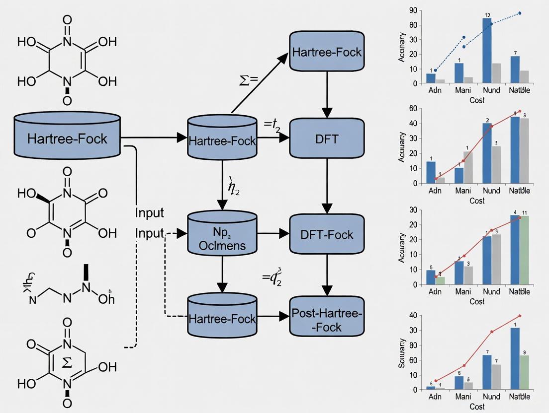
Figure 2: A modern computational NMR workflow for 3D structure determination, showing the integration of theoretical calculations with experimental validation. This iterative process refines structural models until agreement is achieved between computed and observed NMR parameters.

Ramsey's nonrelativistic theory established the fundamental language for describing NMR interactions, creating a formalism that has demonstrated remarkable resilience and adaptability. While modern computational methods have dramatically expanded in sophistication—addressing gauge problems, incorporating relativistic effects, and harnessing machine learning—they remain firmly grounded in the physical insights and mathematical framework first articulated over seven decades ago. The continued development of standardized benchmarking datasets and more efficient computational protocols ensures that this powerful synergy between foundational theory and modern computation will continue to drive advancements in structural biology, drug discovery, and materials science. As computational power grows and algorithms refine, Ramsey's enduring legacy persists as the foundational syntax in the language of NMR parameter computation.

Nuclear Magnetic Resonance (NMR) spectroscopy stands as a cornerstone analytical technique in modern chemical and pharmaceutical research, providing unparalleled insights into molecular structure, dynamics, and interactions. The discovery that nuclear resonance frequencies depend on the chemical environment—the chemical shift—represented a fundamental breakthrough that elevated NMR from a physical phenomenon to an essential analytical tool [6]. At the heart of NMR spectroscopy lies the concept of nuclear magnetic shielding, a tensor property that describes how electrons in a molecule modify the local magnetic field experienced by atomic nuclei. This shielding arises from complex electronic interactions that can be conceptually and computationally separated into two primary components: diamagnetic and paramagnetic shielding contributions [7] [8]. Understanding these contributions is not merely of theoretical interest; it enables researchers to interpret NMR spectra with greater accuracy, validate quantum chemical computations, and ultimately advance drug discovery programs through more reliable structural elucidation.

The theoretical framework for understanding magnetic shielding was established by Ramsey in 1950, who recognized that corrections using only Lamb's diamagnetic theory were inadequate for molecules and developed the necessary theoretical foundation to explain what would become known as the chemical shift [6]. This review examines the fundamental principles of diamagnetic and paramagnetic shielding, compares computational methodologies for their prediction, presents experimental validation protocols, and provides practical guidance for researchers seeking to leverage these concepts in structural biology and pharmaceutical development.

Theoretical Foundations of Magnetic Shielding

The Physical Basis of Nuclear Shielding

When a molecule is placed in an external magnetic field (B₀), the electrons surrounding atomic nuclei generate induced magnetic fields that alter the effective field (B_eff) experienced at the nuclear site. This phenomenon is described by the fundamental shielding relationship:

B_eff = (1 - σ)B₀

where σ represents the shielding constant [7] [8]. In diamagnetic molecules, the overall shielding (σ_i) for a nucleus i can be conceptually decomposed into three components as noted by Saika and Slichter:

σi = σi^d + σi^p + ∑(i≠j)σ_j

where σi^d represents the local diamagnetic contribution, σi^p represents the local paramagnetic contribution, and the final term accounts for modifications arising from both intra- and intermolecular effects [7] [8]. This decomposition provides a powerful framework for understanding how molecular structure and electronic environment influence observed NMR parameters.

Diamagnetic Shielding Contribution

The diamagnetic term (σ_i^d) arises from the circulation of electrons in spherical distributions around the nucleus and always produces a positive contribution to shielding, meaning it reduces the resonant frequency [7] [8]. According to the formulation provided by Pople, this term can be expressed as:

σi^d = (μ₀/4π)(e²/3me)⟨0|∑n(1/rn)|0⟩

where e represents electron charge, me is electron mass, μ₀ is free space permeability, and rn is the distance from the nth electron to an arbitrary origin [7] [8]. The diamagnetic term dominates in atoms with spherical symmetry and is particularly significant for hydrogen atoms, which lack p, d, or f electrons. In molecules, this term responds primarily to local electron density, increasing with greater s-character in bonding orbitals and decreasing with electronegative substituents that withdraw electron density.

Paramagnetic Shielding Contribution

The paramagnetic term (σ_i^p) originates from non-spherical electron distributions, particularly those involving p, d, or f electrons, and always produces a negative contribution (deshielding effect) [7] [8]. This term can be expressed as:

σi^p = -(μ₀/4π)(e²/3me)∑(k≠0)[1/(Ek - E0)]⟨0|∑n Ln|k⟩⟨k|∑n (Ln/rn³)|0⟩

where Ln represents the orbital angular momentum for the nth electron, E0 and E_k are energies of ground and excited states, respectively [7] [8]. The paramagnetic term depends critically on the accessibility of excited states (inverse energy dependence) and the matrix elements connecting these states via angular momentum operators. This term dominates for nuclei in unsymmetrical environments or those with accessible excited states, particularly heavy atoms and atoms involved in multiple bonding.

Tensor Nature of Shielding

Magnetic shielding is fundamentally a second-rank tensor property with nine independent components, meaning the screening of the external magnetic field depends on the relative orientation of the field and the molecule [6]. In single crystals, this orientation dependence manifests as changes in resonance frequencies as the crystal is rotated relative to the magnetic field. For disordered solid samples, this results in characteristic powder patterns, while in liquids, rapid molecular tumbling averages the tensor to its isotropic value:

σiso = 1/3(σxx + σyy + σzz)

The relationship between the shielding tensor (σ) and the experimentally observed chemical shift tensor (δ) is given by:

δ = 1(σ_iso - σ)

where σ_iso represents the isotropic shielding of the reference compound [6]. This tensor nature provides rich structural information in solid-state NMR that is largely lost in solution studies.

Figure 1: Conceptual diagram illustrating how diamagnetic (blue) and paramagnetic (red) shielding contributions modify the external magnetic field to determine the effective field at the nucleus and resulting NMR frequency.

Computational Methodologies for Shielding Prediction

Density Functional Theory (DFT) Approaches

Density Functional Theory has established itself as a cornerstone method for predicting NMR parameters, offering an optimal balance between computational efficiency and accuracy [2]. Most periodic DFT computations in NMR crystallography rely on functionals from the generalized gradient approximation (GGA) family, particularly the Perdew-Burke-Ernzerhof (PBE) functional, which provides reasonable predictions but doesn't always achieve precise agreement with experimental data [9]. The gauge-including projector augmented wave (GIPAW) method was specifically developed for DFT calculations of magnetic resonance properties using pseudopotentials and plane waves as the basis set for wave-function calculations, and has been successfully applied in numerous NMR crystallography studies [9].

For improved accuracy, hybrid functionals such as PBE0 incorporate exact Hartree-Fock exchange, often yielding superior agreement with experimental data. Recent studies have demonstrated that PBE0-based corrections applied to periodic PBE predictions significantly improve agreement with experimental ¹³C chemical shifts, markedly reducing root-mean-square deviations (RMSD) [9]. This approach maintains computational feasibility while achieving accuracy comparable to more expensive computational methods.

Fragment and Cluster Correction Methods

To address limitations in periodic DFT calculations, fragment-based correction methods have been developed that combine the efficiency of periodic calculations with the accuracy of higher-level methods [9]. In this approach:

• Nuclear shieldings are first calculated in the fully periodic crystal structure at the PBE level
• An isolated molecule or molecular fragment is extracted from the periodic structure
• Shielding is computed for the fragment at both PBE level and a higher computational level (e.g., hybrid DFT functional)
• The difference between these calculations serves as a correction to the periodic PBE results

This method has been successfully extended to compute quadrupolar couplings and has demonstrated particular value for predicting ¹³C chemical shifts in organic solids, with later extensions utilizing larger fragments of the crystal structure to compute corrections at higher computational levels [9]. The approach maintains periodic accuracy while incorporating higher-level electronic structure corrections.

Emerging Machine Learning Protocols

Recent machine learning approaches have revolutionized shielding predictions by offering dramatic improvements in computational efficiency. Methods like ShiftML2 can accelerate computations by several orders of magnitude while maintaining accuracy comparable to traditional quantum-chemical methods [9]. These models are trained on diverse structures from crystallographic databases, using shieldings computed at the DFT level with the PBE functional.

Machine learning models have proven particularly valuable for integrating molecular dynamics (MD) simulations with shielding predictions, providing insights into the structure of amorphous materials and enabling the analysis of dynamic systems previously inaccessible to computational NMR [9]. However, unlike traditional quantum chemical methods, ML approaches do not explicitly separate diamagnetic and paramagnetic contributions, instead learning the relationship between structure and total shielding directly from training data.

Table 1: Comparison of Computational Methods for NMR Shielding Prediction

Method	Theoretical Foundation	Accuracy	Computational Cost	Key Applications
GGA-DFT (PBE)	Density Functional Theory	Moderate	Moderate	Initial screening, large systems
Hybrid-DFT (PBE0)	DFT with Hartree-Fock exchange	High	High	Benchmark calculations, final validation
Fragment-Corrected DFT	Combines periodic and molecular calculations	High	Moderate-High	Molecular crystals, pharmaceutical polymorphs
Machine Learning (ShiftML2)	Pattern recognition on DFT training data	Moderate-High	Very Low	High-throughput screening, MD simulations

Experimental Protocols and Validation

Reference Standards and Absolute Shielding Scales

Experimental determination of nuclear magnetic shielding requires careful calibration against reference standards with known absolute shielding values [6]. The relationship between observed chemical shifts (δ) and shielding constants (σ) is defined as:

δi ≈ σref - σ_i

where σ_ref represents the shielding of the reference compound [7] [8]. Primary references are established through sophisticated methods involving gas-phase studies, spin-rotation constants, and theoretical calculations, which are then transferred to practical secondary standards for routine laboratory use.

Table 2: Absolute Shielding Scales for Common NMR Nuclei

Nucleus	Primary Reference	Absolute Shielding (σ_iso)	Common Secondary Reference	Secondary Reference Shielding
¹H	Hydrogen atom	17.733 ppm	Tetramethylsilane (TMS)	~31 ppm (derived)
¹³C	Carbon monoxide	3.20 ppm	TMS	185.4 ppm
¹⁵N	Ammonia	264.54 ppm	Nitromethane	-135.0 ppm
¹⁷O	Carbon monoxide	-42.3 ppm	Water	307.9 ppm
¹⁹F	Hydrogen fluoride	410.0 ppm	CFCl₃	189.9 ppm
³¹P	Phosphine	597.0 ppm	Phosphoric acid	356.0 ppm

Gas-Phase NMR for Isolated Molecule Studies

Gas-phase NMR measurements are crucial for separating intrinsic molecular shielding parameters from intermolecular contributions present in condensed phases [7] [8]. By extrapolating shielding measurements to the zero-density limit, researchers can obtain shielding values (denoted as σ₀) equivalent to isolated molecules [7] [8]. These measurements provide essential benchmarks for quantum chemical calculations, which typically model molecules in isolation without environmental effects.

Experimental protocols for gas-phase NMR require specialized equipment to handle gases at controlled densities and temperatures. Measurements are performed at multiple densities and extrapolated to zero density to eliminate residual intermolecular effects, providing the true isolated molecule shielding [7] [8]. These values allow direct comparison with quantum chemical calculations without the need to model bulk solvent or crystal packing effects.

Validation Data Sets for Method Benchmarking

Comprehensive experimental datasets with validated NMR parameters are essential for benchmarking computational methods. A recent study published over 1000 accurately defined and validated experimental parameters, including 775 proton-carbon scalar coupling constants (ⁿJCH), 300 proton-proton scalar coupling constants (ⁿJHH), 332 ¹H chemical shifts, and 336 ¹³C chemical shifts for fourteen complex organic molecules [3].

The validation process involves comparing experimental NMR parameters with DFT-calculated values to identify potential misassignments. A subset of 565 ⁿJCH, 205 ⁿJHH, 172 ¹H chemical shifts, and 202 ¹³C chemical shifts from rigid portions of these molecules has been identified as particularly valuable for benchmarking computational methods for predicting NMR parameters [3]. These datasets provide robust benchmarks for evaluating the performance of different computational protocols in predicting both shielding constants and coupling parameters.

Figure 2: Experimental workflow for NMR parameter determination and computational validation, showing multiple pathways for gas-phase, solution, and solid-state measurements.

Comparative Performance Analysis

Accuracy Across Nuclear Environments

The performance of computational methods varies significantly across different nuclear environments and elements. Recent studies comparing DFT and machine-learning predictions of NMR shieldings reveal that correction schemes originally developed for periodic DFT calculations can significantly improve agreement with experimental ¹³C chemical shifts [9]. The application of PBE0-based corrections to periodic PBE predictions has markedly reduced RMSD values for carbon nuclei in molecular crystals [9].

In contrast, these corrections demonstrate minimal impact on ¹H shieldings, highlighting the differential sensitivity of various nuclei to computational methodologies [9]. This nuclear dependence reflects the varying contributions of diamagnetic and paramagnetic terms across the periodic table, with proton shielding being dominated by local diamagnetic contributions that are well-described by standard DFT functionals, while heavier elements with significant paramagnetic contributions require more sophisticated treatment.

Performance in Pharmaceutical Applications

In pharmaceutical research, where molecular complexity and conformational flexibility present particular challenges, the mPW1PW91/6-311G(d,p) level of theory has emerged as a valuable compromise between accuracy and computational feasibility [3]. This approach has been successfully applied to compute magnetic shielding tensors that are subsequently converted to experimentally relevant chemical shifts through scaling procedures.

The availability of validated experimental datasets has enabled systematic benchmarking of these computational protocols, revealing their strengths and limitations for different molecular classes [3]. For rigid substructures, modern DFT methods can achieve remarkable accuracy, while flexible regions remain challenging due to the need for extensive conformational sampling and the sensitivity of shielding to precise molecular geometry.

Table 3: Key Computational and Experimental Resources for NMR Shielding Research

Resource Category	Specific Tools/Methods	Primary Function	Key Applications
Quantum Chemical Software	Gaussian, ORCA, CP2K, Quantum ESPRESSO	Shielding tensor calculation	Method development, benchmark calculations
Machine Learning Protocols	ShiftML2, Impression	Fast shielding prediction	High-throughput screening, MD integration
Reference Standards	TMS, DSS, Adamantane	Chemical shift referencing	Experimental calibration
Specialized NMR Experiments	IPAP-HSQMBC, EXSIDE	Scalar coupling measurement	Stereochemical analysis, conformation determination
Validation Datasets	C4X Discovery dataset [3]	Method benchmarking	Computational protocol validation
Solid-State NMR Methods	GIPAW DFT, Fragment corrections	Crystal structure refinement	NMR crystallography, polymorph characterization

The deconstruction of NMR parameters into diamagnetic and paramagnetic shielding contributions provides not only fundamental theoretical insights but also practical advantages for method development and applications in structural science. While DFT remains the workhorse for shielding predictions, the emergence of machine learning protocols promises to dramatically expand the scope and scale of computational NMR applications [9] [2].

The ongoing refinement of fragment-based correction schemes offers a promising pathway to accuracy competitive with high-level quantum chemical methods at substantially reduced computational cost [9]. As validation datasets continue to expand and diversify, particularly for pharmaceutically relevant compounds [3], researchers are better equipped than ever to select appropriate computational strategies for specific applications.

Future developments will likely focus on improving accuracy for challenging nuclei, extending methods to dynamic systems, and enhancing integration with experimental structural biology workflows. The continued synergy between theoretical advances, computational innovations, and experimental validation ensures that NMR shielding analysis will remain an indispensable tool for molecular structure elucidation across chemistry, materials science, and drug discovery.

A fundamental challenge in the theoretical calculation of Nuclear Magnetic Resonance (NMR) parameters is the gauge invariance problem. In quantum chemical calculations, the computed NMR chemical shielding constants should be independent of the chosen coordinate system. However, in practice, when finite basis sets are used, the results can become gauge-dependent, meaning that the calculated NMR chemical shifts artificially vary with the origin chosen for the magnetic vector potential. This problem is particularly pronounced in calculations on large molecules or those involving heavy elements, where gauge errors can lead to significant inaccuracies that compromise the predictive value of the computations.

The gauge invariance problem arises because the presence of an external magnetic field introduces a vector potential into the quantum mechanical Hamiltonian. The exact solution to this Hamiltonian would naturally be gauge-invariant, but the use of localized atomic orbital basis sets breaks this inherent invariance. This creates a critical methodological hurdle that must be overcome to achieve chemically accurate NMR predictions, especially for applications in drug development and materials science where reliable computational predictions can guide expensive synthetic efforts. The development of robust solutions to this problem has been a central focus in computational NMR for decades, leading to several sophisticated theoretical approaches.

The Gauge-Including Atomic Orbital (GIAO) Approach

The Gauge-Including Atomic Orbital (GIAO) method, also known as London Atomic Orbitals, represents the most widely adopted solution to the gauge invariance problem in computational chemistry. The fundamental innovation of the GIAO approach involves constructing basis functions that explicitly include the magnetic field vector potential. A GIAO basis function χ is defined as χ_μ(B) = exp[(-i/2c)(B × R_μ) ⋅ r] ⋅ χ_μ(0), where χ_μ(0) is the standard field-independent atomic orbital, B is the magnetic field vector, R_μ is the position vector of the basis function's center, and r is the electron coordinate vector. This complex phase factor ensures that each atomic orbital transforms correctly under gauge transformations, making the overall wavefunction and the resulting NMR shieldings intrinsically gauge-invariant.

The GIAO method has been successfully implemented in numerous quantum chemistry packages, including the ADF software platform, where it serves as the foundation for NMR chemical shift calculations [10]. The implementation requires careful handling of both the diamagnetic and paramagnetic contributions to the shielding tensor. For practical computation, the ADF implementation requires both the adf.rkf (TAPE21) result file and a TAPE10 file that contains the SCF potential from an initial ADF calculation [10]. The GIAO method's principal advantage lies in its rapid convergence with basis set size compared to alternative approaches, typically delivering accurate results with relatively compact basis sets.

Table 1: Key Features of the GIAO (Gauge-Including Atomic Orbital) Approach

Feature	Description	Implication for NMR Calculations
Basis Set Dependence	Complex basis functions with field-dependent phase factors	Reduces gauge origin error, faster convergence with basis set size
Implementation Complexity	Requires modification of Hamiltonian and integral derivatives	Computationally demanding but highly accurate
Relativistic Compatibility	Compatible with ZORA and spin-orbit treatments [10]	Suitable for heavy elements and organometallic complexes
Systematic Improvement	Accuracy improves with basis set quality and DFT functional	Predictable path to higher accuracy through computational cost

Alternative Modern Approaches to Gauge Invariance

While GIAO represents the gold standard, several alternative approaches have been developed to address the gauge invariance problem, each with distinct advantages and limitations.

The Continuous Set of Gauge Transformations (CSGT) method represents an important alternative strategy. Rather than using field-dependent basis functions, CSGT calculates the shielding tensor at each point in space using a different gauge origin chosen specifically for that point—typically the point itself. This distributed gauge origin approach effectively eliminates gauge dependence but requires careful numerical integration over molecular space. CSGT implementations often leverage density functional theory and have been shown to produce results comparable to GIAO for many organic molecules, though they may exhibit different performance for metallic systems or molecules with complex electron delocalization.

The Individual Gauge for Localized Orbitals (IGLO) approach constitutes another significant methodology. IGLO uses localized molecular orbitals and assigns each orbital its own gauge origin, typically chosen at the orbital's center. This method can be computationally efficient for small to medium-sized molecules but may face challenges in systems where orbital localization is difficult or ambiguous. The performance of IGLO can be sensitive to the localization procedure employed, potentially introducing methodological dependencies that are less pronounced in the GIAO approach.

Comparative Performance of Modern Methods

The relative performance of different gauge-invariant methods depends critically on the chemical system under investigation, the chosen computational parameters, and the specific NMR parameters of interest. The table below summarizes a qualitative comparison of the most widely used approaches.

Table 2: Comparison of Gauge-Invariant Methods for NMR Chemical Shift Calculations

Method	Gauge Handling Approach	Computational Cost	Best Application Areas	Key Limitations
GIAO	Field-dependent complex atomic orbitals	High (efficient with modern algorithms)	Universal application, heavy elements, aromatic systems [10]	Implementation complexity; requires analytical derivatives
CSGT	Distributed gauge origins in real space	Moderate to High	Organic molecules, main-element chemistry	Integration sensitivity for metallic systems
IGLO	Individual gauges for localized orbitals	Moderate	Small to medium organic molecules	Performance depends on localization scheme

When implementing these methods within density functional theory, the choice of exchange-correlation functional introduces another dimension of variability. For instance, the SAOP potential has been shown to yield "isotropic chemical shifts which are substantially improved over both LDA and GGA functionals" according to ADF documentation [10]. However, certain computational restrictions apply, as "Meta-GGA's and meta-hybrids should not be used in combination with NMR chemical shielding calculations" in the ADF implementation due to incorrect inclusion of GIAO terms [10].

Experimental Protocols and Computational Methodologies

Standard Protocol for GIAO-NMR Calculations

A robust workflow for calculating NMR chemical shifts using the GIAO approach involves several critical steps that ensure gauge-invariant, chemically accurate results:

• Molecular Geometry Optimization: Begin with a carefully optimized molecular geometry using an appropriate level of theory (e.g., DFT with a functional such as B3LYP and a basis set like def2-TZVP).
• Single-Point Energy Calculation: Perform a single-point energy calculation on the optimized structure using ADF with the keyword SAVE TAPE10 to store the SCF potential [10].
• NMR Calculation Setup: Execute the NMR property module using the generated adf.rkf (TAPE21) and TAPE10 files as input [10].
• Relativistic Treatment Selection: For heavy elements, incorporate relativistic effects using the ZORA Hamiltonian, ensuring consistent use of either scaled or unscaled approaches throughout the study [10].
• Reference Compound Calculation: Compute the shielding constant for a reference compound (e.g., TMS for 1H and 13C) using identical computational parameters.
• Chemical Shift Derivation: Calculate the final chemical shift δ_i for nucleus i using the formula δ_i = σ_ref - σ_i, where σ_ref and σ_i are the shielding constants of the reference and target nuclei, respectively [10].

The following workflow diagram illustrates the standard protocol for GIAO-NMR calculations:

Special Considerations for Heavy Elements

For systems containing heavy elements, additional theoretical considerations become crucial. The ADF documentation specifically notes that "NMR calculations on systems computed by ADF with Spin Orbit relativistic effects included must have used NOSYM symmetry in the ADF calculation" [10]. Furthermore, an "improved exchange-correlation kernel, as was implemented by J. Autschbach" can be activated using the USE FXC keyword, which is particularly important for spin-orbit coupled calculations [10]. These technical details highlight the sophisticated treatment required for heavy elements, where relativistic effects significantly influence NMR parameters.

Implementing gauge-invariant NMR calculations requires access to specialized software tools and methodological components. The following table details essential "research reagent solutions" for computational chemists working in this domain.

Table 3: Essential Computational Tools for Gauge-Invariant NMR Calculations

Tool Category	Specific Examples	Function in NMR Research
Quantum Chemistry Software	ADF [10], Gaussian, ORCA	Provides implementations of GIAO, CSGT, and other gauge-invariant methods
Relativistic Methods	ZORA (scaled/unscaled) [10], Spin-Orbit coupling	Accounts for relativistic effects critical for heavy elements
Exchange-Correlation Functionals	SAOP [10], GGA, Hybrid Functionals	Determines accuracy of NMR shielding predictions; some functionals have restrictions
Basis Sets	Slater-type orbitals, Gaussian-type orbitals	Basis set quality and completeness directly impact gauge invariance and accuracy
Analysis Modules	NBO analysis, shielding tensor visualization [10]	Enables interpretation of NMR parameters in terms of chemical structure

The gauge invariance problem in computational NMR has been largely addressed through sophisticated theoretical approaches, with the Gauge-Including Atomic Orbital (GIAO) method emerging as the most robust and widely adopted solution. Its compatibility with relativistic treatments like ZORA and consistent performance across diverse chemical systems make it particularly valuable for pharmaceutical and materials science applications where predictive accuracy is paramount. While alternative methods like CSGT and IGLO offer valuable insights and occasionally computational advantages for specific systems, GIAO remains the benchmark for comprehensive NMR parameter prediction.

Future methodological developments will likely focus on enhancing the computational efficiency of gauge-invariant calculations for large biomolecular systems, improving the treatment of environmental effects through explicit solvation models, and refining relativistic methodologies for increasingly heavy elements. As quantum chemical methods continue to evolve alongside computational hardware, the integration of gauge-invariant NMR prediction into automated workflow tools will further expand its utility in drug discovery and materials characterization, solidifying its role as an indispensable component of the modern computational chemist's toolkit.

Relativistic quantum chemistry combines the principles of relativistic mechanics with quantum chemistry to accurately calculate the properties and structure of elements, particularly the heavier members of the periodic table [11]. For much of the history of quantum mechanics, relativistic effects were considered negligible for chemical systems, a sentiment famously echoed by Paul Dirac in 1929 [11]. However, since the 1970s, it became clear that this assumption fails for heavy elements, where electrons, especially those in s and p orbitals, attain significant velocities relative to the speed of light [11] [12]. Relativistic effects are formally defined as the discrepancies between values calculated by models that incorporate relativity and those that do not [11]. These effects are no longer mere curiosities but are essential for explaining fundamental chemical behaviors, from the color of gold and the liquidity of mercury at room temperature to the performance of lead-acid batteries [11] [12].

Within the specific context of Nuclear Magnetic Resonance (NMR) parameters, relativistic effects become critically important. The presence of a heavy atom in a molecule can profoundly influence the NMR chemical shifts and spin-spin coupling constants, both for itself and for nearby light atoms [13] [14]. Accurately computing these parameters for systems containing heavy elements necessitates a relativistic quantum mechanical treatment, making this a central focus in modern computational chemistry methodologies for NMR research [14].

When Relativistic Effects Matter: Key Elements and Phenomena

Relativistic effects grow roughly with the square of the atomic number (Z²), becoming substantial for elements in the 6th period and dominant in the 7th period of the periodic table [12]. The following table summarizes key elements and properties where relativistic effects are most pronounced.

Table 1: Elemental Systems and Properties Significantly Influenced by Relativistic Effects

Element/System	Property Influenced	Non-Relativistic Expectation	Relativistic Reality
Gold (Au)	Color	Silvery, like copper and silver [11]	Yellow/Golden due to blue light absorption [11]
Mercury (Hg)	Physical State	Solid at room temperature, like cadmium [11]	Liquid metal (m.p. -39°C) [11]
Caesium (Cs)	Color	Silver-white, like other alkali metals [11]	Pale golden yellow [11]
Lead-Acid Battery	Voltage	Behaves like tin, low voltage [11] [12]	~12 V (10 V from relativistic effects) [11] [12]
Thallium (Tl), Lead (Pb), Bismuth (Bi)	Oxidation Chemistry	Stable +3, +4, +5 states, respectively [11]	Inert-pair effect: Stable +1, +2, +3 states [11]
Lanthanides	Atomic Radius	Gradual decrease (Lanthanide Contraction)	~10% of the contraction is relativistic in origin [11]
Superheavy Elements (Rf-Og)	Chemical Properties	Extrapolated from lighter congeners [12]	Chemistry is "predominantly controlled" by relativity [12]

The qualitative understanding of these phenomena stems from two primary relativistic corrections: the mass-velocity correction and spin-orbit coupling. The mass-velocity correction accounts for the increase in electron mass as its speed approaches the speed of light, given by (m{\text{rel}} = me / \sqrt{1 - (v_e/c)^2}) [11]. This leads to a contraction and stabilization of s and p orbitals (direct relativistic effect) [12]. Consequently, orbitals with higher angular momentum (d and f orbitals) become more shielded from the nuclear charge and expand (indirect relativistic effect) [12]. Spin-orbit (SO) coupling, the third major relativistic effect, splits orbitals with non-zero angular momentum (e.g., p, d, f) into subsets with different total angular momentum (e.g., p₁/₂ and p₃/₂), further complicating the electronic structure of heavy atoms [12] [15].

Diagram: The Primary Mechanisms of Relativistic Effects in Heavy Atoms

Relativistic Effects on NMR Parameters: The HALA and HAHA Phenomena

In NMR spectroscopy, relativistic effects are not just a minor correction but a dominant factor for systems containing heavy atoms. Two key phenomena are observed:

• HALA (Heavy Atom on Light Atom Effect): The presence of a heavy atom can significantly shift the NMR chemical shifts of nearby light nuclei (e.g., ¹H, ¹³C, ¹⁵N, ¹⁹F) [13] [14]. This is primarily due to the spin-orbit coupling term of the heavy atom, which polarizes the electron density and alters the shielding of the light nucleus [14].
• HAHA (Heavy Atom on Heavy Atom Effect): Relativistic effects also dramatically alter the NMR parameters of the heavy atoms themselves, such as ¹⁹⁹Hg, ¹⁹⁵Pt, ²⁰⁷Pb, and halogens [16] [17]. For these nuclei, scalar relativistic effects (mass-velocity and Darwin terms) are often the dominant contributors to their chemical shifts, though spin-orbit coupling can also play a major role [17].

The importance of these effects is starkly illustrated in the hydrogen halide series (HF, HCl, HBr, HI). The experimental ¹H NMR chemical shift changes dramatically down the group, a trend that can only be reproduced computationally by including spin-orbit relativistic corrections [13]. Similarly, for ¹⁹⁹Hg, non-relativistic computational methods fail to reproduce experimental chemical shifts, while relativistic methods like ZORA (Zeroth-Order Regular Approximation) show excellent agreement, enabling the use of ¹⁹⁹Hg NMR as a robust structural descriptor [17].

Comparative Performance of Quantum Chemical Methods for NMR

The accurate calculation of NMR parameters in heavy-element systems requires methods that incorporate relativistic corrections. The table below compares the performance of different computational approaches.

Table 2: Comparison of Quantum Chemical Methods for Relativistic NMR Parameter Calculation

Computational Method	Relativistic Treatment	Typical Application Scope	Performance & Notes
Zeroth-Order Regular Approximation (ZORA)	Scalar Relativistic (SR) or Spin-Orbit (SO) [13]	Molecules with heavy atoms (e.g., I, At, Hg) [16] [13] [17]	Excellent performance for ¹H shifts in H-X; SR good for structural trends, SO essential for accurate shifts [13]. Efficient and widely used.
Dirac–Kohn–Sham (Four-Component)	Full Relativistic [14]	Benchmark calculations; systems with extreme relativistic effects [18] [14]	The most theoretically rigorous approach. High computational cost but serves as a gold standard [18].
Relativistic Effective Core Potentials (RECPs)	Implicit (via pseudopotential) [15]	Large systems where full relativity is prohibitive [15]	Reduces computational cost by replacing core electrons. Accuracy depends on pseudopotential quality [15].
Douglas-Kroll-Hess (DKH)	Scalar Relativistic [15]	Medium-to-large molecules with heavy atoms [15]	High accuracy for scalar properties. More approximate than four-component methods but more efficient [15].
Non-Relativistic Hamiltonian	None	Light elements (Z < ~30) only [16]	Fails qualitatively for NMR parameters of heavy atoms and their light neighbors (e.g., HALA effect) [16] [13].

The choice of methodology is critical. For instance, a study on halogen-bonded complexes showed that relativistic corrections are essential for calculating NMR parameters when involving iodine and astatine, with the ZORA Hamiltonian providing the necessary accuracy [16]. Furthermore, a 2025 study on mercury-DOTAM complexes demonstrated that relativistic cluster-based methods (ADF/ReSpect) significantly outperformed non-relativistic approaches for calculating ¹⁹⁹Hg NMR shifts [17].

Diagram: Workflow for Relativistic Computation of NMR Parameters

Experimental Protocols and Research Toolkit

Protocol: Relativistic DFT Calculation of NMR Shifts

This protocol outlines the steps for calculating NMR chemical shifts using relativistic Density Functional Theory (DFT), as demonstrated for the hydrogen halides and mercury complexes [13] [17].

• Geometry Optimization: Pre-optimize the molecular structure using a relativistic method. For accurate NMR results, this can be done at the ZORA scalar relativistic level.

  • Functional: A hybrid functional like PBE0 is recommended for better accuracy, though GGA functionals like PBE can be used for faster results [13].
  • Basis Set: Use an all-electron triple-zeta or quadruple-zeta basis set (e.g., QZ4P, TZ2P) on all atoms, especially those for which NMR parameters are desired [13].
  • Relativistic Hamiltonian: Select ZORA (scalar or spin-orbit) [13].
  • Numerical Quality: Set to "Good" to ensure accurate integration grids [13].

• Single-Point NMR Calculation: Using the optimized geometry, perform a single-point energy calculation with the focus on NMR properties.

  • Functional and Basis Set: Consistent with the optimization step. Using QZ4P is recommended for high accuracy [13].
  • Relativistic Treatment: For final NMR values, the ZORA spin-orbit Hamiltonian is often necessary to capture the full relativistic effect, especially for the HALA effect and heavy atom shifts [13].
  • Property Calculation: Request the calculation of isotropic shielding constants and full shielding tensors for the nuclei of interest.

• Chemical Shift Referencing: Convert the calculated absolute shielding constants (σᵢ) to the experimental chemical shift scale (δᵢ) using a reference compound: δᵢ = σref - σᵢ. For example, in the hydrogen halide series, HF is used as the reference (δ(¹H) = 0.0 ppm, σref = 28.72 ppm) [13].

The Scientist's Toolkit for Relativistic NMR

Table 3: Essential Computational Tools and Concepts for Relativistic NMR Studies

Tool/Concept	Function & Purpose	Example Use-Case
ZORA Hamiltonian	An efficient method to approximate the solution to the Dirac equation; can be applied in scalar (SR) or spin-orbit (SO) forms [13] [15].	Calculating the ¹H NMR shift in HI, where SO effects are crucial for accuracy [13].
Relativistic DFT Functionals (PBE0, PB86)	The exchange-correlation functionals used in conjunction with relativistic Hamiltonians to describe electron interaction. Hybrid functionals (PBE0) generally offer better accuracy [13].	Geometry optimization and NMR property calculation for the W@Au₁₂ cluster [18].
All-Electron Basis Sets (QZ4P, TZ2P)	High-quality basis sets that explicitly describe all electrons in the system, necessary for accurate property calculations on heavy atoms [13].	Achieving quantitative agreement with experimental ¹³C and ¹⁵N shifts in Hg-complexes [17].
Relativistic Effective Core Potentials (RECPs)	Pseudopotentials that replace the core electrons of a heavy atom, incorporating relativistic effects implicitly to reduce computational cost [15].	Modeling the electronic structure of large gold nanoclusters or actinide complexes [18] [15].
Energy Decomposition Analysis (EDA)	A method to decompose interaction energies into components (electrostatic, Pauli repulsion, orbital interaction) to understand bonding [16].	Analyzing the nature of halogen bonds in complexes involving heavy halogens like At [16].

Relativistic effects are not peripheral concerns but central determinants of the chemical and spectroscopic behavior of heavy elements. For researchers relying on NMR spectroscopy, ignoring these effects leads to qualitatively and quantitatively incorrect results. The development of efficient and accurate relativistic methods like ZORA and DKH within quantum chemical software has moved these tools from specialist domains to essential components of the computational chemist's arsenal. As research pushes further into the chemistry of superheavy elements and complex heavy-atom materials, and as the demand for precise structural elucidation in drug discovery and materials science grows, the role of relativistic quantum chemistry in predicting and interpreting NMR parameters will only become more critical. The continued refinement of these methods ensures that scientists have the necessary tools to explore the fascinating and non-intuitive chemistry governed by Einstein's theory of relativity.

In the field of computational chemistry, the prediction of Nuclear Magnetic Resonance (NMR) parameters relies on sophisticated quantum chemical methods that balance theoretical accuracy with computational feasibility. The virial theorem and the concept of the complete basis set (CBS) limit represent two fundamental approximations that profoundly impact the reliability of these predictions. The virial theorem governs the relationship between kinetic and potential energy in molecular systems, providing a critical check on wavefunction quality, while the CBS limit represents the theoretical target where properties become independent of basis set size. Understanding these approximations is particularly crucial for researchers and drug development professionals who depend on computational NMR for structural elucidation of complex biological molecules, metallopharmaceuticals, and novel materials.

This guide provides a comprehensive comparison of quantum chemical methods for NMR parameters research, examining how different theoretical approaches navigate the trade-offs between accuracy and computational cost. We evaluate performance across multiple methodologies, from Density Functional Theory (DFT) to wavefunction-based approaches, focusing specifically on their application to NMR chemical shift predictions in biologically relevant systems.

Theoretical Framework

The Complete Basis Set Limit in NMR Calculations

The complete basis set limit represents an idealized state where the calculated molecular properties become invariant to further expansion of the basis set. For NMR parameters, particularly chemical shielding tensors, approaching this limit is essential for obtaining results comparable to experimental data. The chemical shift (δ) is a dimensionless parameter representing the relative resonance frequency of nuclei in a sample compared to a reference standard, defined as the ratio of the frequency difference to the spectrometer's operating frequency [2].

Different quantum chemical methods approach the CBS limit at varying rates. Hartree-Fock (HF) methods show poor convergence behavior, with studies demonstrating that "HF values show quite a different tendency to MP2, and even in the CBS limit they are far from experiment for not only the isotropic shielding of carbonyl carbon but also most shielding anisotropies" [19]. In contrast, Møller-Plesset perturbation theory (MP2) demonstrates superior performance, with "MP2 results in the CBS limit show[ing] the best agreement with experiment" for chemical shielding tensors in peptide systems [19].

Interestingly, Density Functional Theory (DFT) exhibits unique behavior in basis set convergence. Research indicates that "small basis-set (double- or triple-zeta) results are often fortuitously in better agreement with the experiment than the CBS ones" due to systematic errors in functionals that partially cancel with basis set incompleteness errors [19]. This phenomenon complicates method selection for NMR parameter prediction.

The Virial Theorem in Electronic Structure Methods

The virial theorem establishes a fundamental relationship between kinetic (T) and potential (V) energy in molecular systems: 2T + V = 0 for atoms and molecules at equilibrium geometries. This theorem serves as a critical quality metric for wavefunctions - deviations from this relationship indicate inadequate description of electron correlation or basis set incompleteness.

While not explicitly discussed in the search results, the implications of the virial theorem underpin the reliability of all quantum chemical methods for NMR parameter prediction. Methods that better satisfy the virial theorem typically provide more accurate electronic distributions, which directly impacts the precision of calculated NMR parameters like chemical shifts and coupling constants. The theorem is particularly relevant when employing embedded or hybrid methods like ONIOM, where consistency between different theoretical levels is essential for accurate property predictions.

Comparative Analysis of Quantum Chemical Methods

Performance Evaluation of Theoretical Methods

Table 1: Performance Comparison of Quantum Chemical Methods for NMR Parameters

Method	Theoretical Foundation	Basis Set Convergence	NMR Parameter Accuracy	Computational Cost	Ideal Application Scope
HF	Wavefunction theory	Slow, poor convergence	Poor for shielding anisotropies [19]	Moderate	Small molecules, educational applications
DFT	Electron density	Variable, error cancellation with small basis sets [19]	Good with selected functionals [2] [20]	Moderate to High	Medium to large systems, transition metals
MP2	Electron correlation	Excellent, best in CBS limit [19]	Highest for peptides [19]	High	Small to medium biomolecules
Coupled-Cluster	High-level correlation	Excellent but expensive [2]	Reference quality [2]	Very High	Benchmark calculations

Table 2: DFT Functional Performance for 49Ti NMR Chemical Shift Prediction

Functional	Basis Set	Relativistic Treatment	Mean Absolute Deviation (ppm)	R²	Computational Cost
OLYP [20]	NMR-DKH (newly developed)	DKH2	48	0.9888	Moderate
4c-BLYP [20]	dyall.VDZ	4-component relativistic	62	0.9860	High
cM06L [20]	pcSseg-3	Not specified	Good but not quantified	Not specified	Very High
B3LYP [20]	6-31G(d)	Non-relativistic	67-110	Not specified	Low
BPW91 [20]	Not specified	Non-relativistic	127	Not specified	Low

Basis Set Selection Strategies

The choice of basis set significantly impacts the accuracy of NMR parameters. Specialized basis sets have been developed for specific applications:

• NMR-DKH basis sets: Specifically designed for NMR calculations with relativistic corrections, these basis sets have shown excellent performance for transition metals including Ti, Pt, Tc, and Co [20]. The recently developed Ti NMR-DKH basis set provides "excellent agreement with experimental data and with lower computational cost" compared to full 4-component relativistic approaches [20].

• Mixed basis set approach: This strategy employs different basis sets for different parts of the molecule, offering superior performance to ONIOM methods for chemical shielding calculations. Research shows "the mixed basis set method provides better results than ONIOM, compared to CBS calculations using the nonpartitioned full systems" for peptide fragments [19].

• Complete basis set extrapolation: For the highest accuracy, CBS extrapolation techniques can be applied, particularly with MP2 methods which show the best performance in the CBS limit for peptide systems [19].

Experimental Protocols and Methodologies

Protocol for Transition Metal NMR Parameters

The accurate prediction of NMR parameters for transition metals requires careful method selection and validation. For titanium-49 NMR chemical shifts, the following protocol has demonstrated excellent performance:

• Geometry Optimization: Optimize molecular structures at the BLYP/def2-SVP level with implicit solvation using IEF-PCM (UFF) model [20].

• Chemical Shift Calculation: Compute NMR chemical shifts at the GIAO-OLYP/NMR-DKH level with the same implicit solvation model [20].

• Relativistic Treatment: Apply second-order Douglas-Kroll-Hess (DKH2) relativistic corrections through the specially designed NMR-DKH basis set [20].

• Validation: Compare calculated values against experimental data using [TiCl₄] as reference compound, with expected chemical shift range from -1389 to +1325 ppm [20].

This protocol achieves a mean absolute deviation of only 48 ppm with a coefficient of determination (R²) of 0.9888 across 41 Ti(IV) complexes, outperforming more computationally expensive 4-component relativistic approaches [20].

Protocol for Biomolecular NMR Parameters

For peptide and protein systems, different considerations apply:

• Method Selection: MP2 methods in the CBS limit provide the best agreement with experiment for chemical shielding tensors in peptide fragments [19].

• Basis Set Strategy: Employ mixed basis set approaches rather than ONIOM methods for more accurate results [19].

• Error Awareness: Recognize that DFT with small basis sets may show fortuitous agreement with experiment due to error cancellation, which doesn't persist at the CBS limit [19].

• Validation Metrics: Assess both isotropic shielding and shielding anisotropy for comprehensive evaluation of method performance [19].

Research Reagent Solutions

Table 3: Essential Computational Tools for NMR Parameter Prediction

Tool/Resource	Type	Function	Application Example
NMR-DKH Basis Sets [20]	Specialized basis sets	Provides accurate NMR parameters with relativistic corrections	Transition metal NMR chemical shifts
GIAO Method [20]	Computational approach	Gauge-including atomic orbitals for origin-independent chemical shifts	NMR parameters in diverse molecular systems
IEF-PCM [20]	Solvation model	Implicit solvation treatment for solution-phase NMR	Biological molecules in aqueous environments
SIMPSON [2]	Simulation package	Models pulse sequences and anisotropic interactions	Solid-state NMR of powdered samples
Spinach Library [2]	Simulation library	Large-scale Liouville space reductions for efficient NMR simulation	Complex spin systems in solution and solid state

Workflow and Method Selection Strategy

(NMR Parameter Prediction Workflow)

The accurate prediction of NMR parameters requires careful consideration of key approximations, particularly the complete basis set limit and the implications of the virial theorem. Our comparison reveals that method performance is highly system-dependent:

For transition metal complexes, specialized protocols using DFT with NMR-DKH basis sets provide excellent accuracy at moderate computational cost, significantly outperforming more expensive 4-component relativistic approaches for Ti-49 NMR chemical shifts [20].

For peptide and protein systems, MP2 methods in the complete basis set limit deliver superior performance for chemical shielding tensors, while DFT exhibits unusual behavior where small basis sets sometimes provide fortuitously better agreement due to error cancellation [19].

For drug development applications, where both organic fragments and metallopharmaceuticals are relevant, a multi-strategy approach is essential. The mixed basis set method offers advantages over ONIOM for fragment-based calculations, providing better balance between accuracy and computational efficiency [19].

These findings underscore the importance of selecting appropriate theoretical methods matched to specific chemical systems, rather than seeking a universal approach. The continuing development of specialized basis sets and computational protocols promises further enhancements in the accuracy and efficiency of NMR parameter prediction for pharmaceutical research and structural biology.

Methodologies in Practice: DFT, Wavefunction, and Hybrid Approaches for Biomolecules

Density Functional Theory (DFT) has established itself as the predominant quantum chemical method for predicting Nuclear Magnetic Resonance (NMR) parameters in medium-to-large molecules, occupying a crucial niche between highly accurate but computationally expensive ab initio methods and faster but less reliable empirical approaches. This balance of reasonable computational cost and acceptable accuracy makes DFT particularly valuable for researchers studying molecular structures of chemical and biological relevance. The method's significance stems from its ability to calculate electronic properties that directly influence NMR parameters, connecting molecular geometry to spectroscopic observables through quantum mechanical principles. While DFT is fundamentally an exact theory, its practical application requires approximations in the exchange-correlation functional, making the choice of functional critical for achieving reliable results [21].

The importance of DFT in molecular sciences is evidenced by its penetration across chemistry, physics, and biology, with the 1998 Nobel Prize awarded to Walter Kohn for its development [21]. For NMR parameter prediction, DFT serves as a pivotal tool that enables researchers to interpret complex spectra, validate molecular structures, and gain insights into electronic environments that experimental data alone cannot provide. This guide examines DFT's performance against alternative methods, providing experimental data and protocols to inform researchers' computational strategies.

Core Theoretical Framework

DFT calculates molecular electronic structure by determining the electron density rather than solving the many-electron wavefunction, significantly reducing computational complexity. For NMR parameters, the method computes nuclear shielding tensors and indirect spin-spin coupling constants, which correlate with experimental chemical shifts and J-couplings. The fundamental workflow involves two sequential calculations: geometry optimization followed by NMR parameter prediction using the gauge-including atomic orbital (GIAO) method, which ensures results are independent of the coordinate system choice [22] [23].

The accuracy of DFT-derived NMR parameters strongly depends on the selected exchange-correlation functional and basis set. Benchmarks across multiple studies reveal that no single functional performs optimally for all nuclei or molecular systems, requiring researchers to match computational methods to their specific applications [24] [22]. Solvation effects must be incorporated through implicit solvent models like the Polarizable Continuum Model (PCM) or Solvation Model based on Density (SMD) to approximate solution-phase conditions [22] [23].

Standard Computational Protocols

Geometry Optimization Protocol:

• Method: B3LYP-D3/6-311G(d,p) level theory, including dispersion correction D3 [22]
• Solvation: Polarizable Continuum Model (PCM) with chloroform parameters [22] [23]
• Conformational Sampling: Generate multiple conformers using ETKDG method, optimize with MMFF94 force field, then apply DFT optimization to low-energy structures [23]
• Validation: Frequency calculations to confirm optimized structures represent true minima (no imaginary frequencies)

NMR Parameter Calculation Protocol:

• Method: Gauge-Independent Atomic Orbital (GIAO) approach [22] [23]
• Functional: ωB97X-D/def2-SVP for 13C NMR; WP04/6-311++G(2d,p) for 1H NMR [22]
• Solvation: Include solvent effects consistently with optimization step [23]
• Reference: Use linear scaling relative to tetramethylsilane (TMS) calculated at same level of theory [22]

The following diagram illustrates the complete DFT workflow for NMR parameter prediction:

Performance Comparison: DFT vs. Alternative Methods

Quantitative Accuracy Assessment

Table 1: Performance Comparison of NMR Prediction Methods for Organic Molecules

Method Category	Specific Method	1H δ MAE (ppm)	13C δ MAE (ppm)	Computational Cost	System Size Limit
DFT (Recommended)	ωB97X-D/def2-SVP	0.07-0.19	0.5-2.9	Hours to days	~100 atoms
DFT (Cs compounds)	rev-vdW-DF2	N/A	N/A	Similar to above	Similar to above
Machine Learning	IMPRESSION-G2	0.07	0.8	Milliseconds	~1000 g/mol
Machine Learning	CSTShift	0.078-0.185	0.504-0.944	Seconds	~64 atoms
Coupled Cluster	CCSD(T)	<0.05	<0.3	Days to weeks	~20 atoms
Empirical	HOSE codes	0.1-0.3	1-3	Milliseconds	No limit

MAE = Mean Absolute Error compared to experimental values; N/A = Data not available in search results for this specific nucleus [22] [23] [25].

Application-Specific Performance

DFT's performance varies significantly across different nuclear environments and molecular systems. For light atoms (1H, 13C) in organic molecules, well-validated functionals like WP04 and ωB97X-D achieve experimental accuracy of 0.07-0.19 ppm for 1H and 0.5-2.9 ppm for 13C chemical shifts [22]. For heavier nuclei like 133Cs, specialized functionals including rev-vdW-DF2 and PBEsol+D3 provide optimal geometry and chemical shift prediction for nuclear waste immobilization studies [24].

For J-coupling constants, which are more sensitive to three-dimensional geometry, DFT methods can predict 3JHH couplings with accuracy approaching 0.15 Hz when appropriate functionals and basis sets are employed [25]. The method's ability to naturally include electron correlation effects, albeit approximately, makes it superior to Hartree-Fock for properties dependent on subtle electronic distribution changes.

Emerging Alternatives: Machine Learning Challenges

Machine learning (ML) approaches represent the most significant emerging challenge to DFT's dominance in NMR prediction. These methods learn the relationship between molecular structure and NMR parameters from large DFT-computed or experimental datasets, achieving remarkable speed improvements. The IMPRESSION-G2 model predicts approximately 5000 chemical shifts and scalar couplings per molecule in <50 milliseconds – approximately 10^6-times faster than DFT calculations starting from 3D structures [25].

When combined with fast GFN2-xTB geometry optimizations, complete ML workflows for NMR predictions are 10^3-10^4 times faster than wholly DFT-based workflows while maintaining comparable accuracy [25]. Similarly, the CSTShift model, a 3D graph neural network incorporating DFT-calculated shielding tensor descriptors, achieves mean absolute errors of 0.078-0.185 ppm for 1H and 0.504-0.944 ppm for 13C chemical shifts on benchmark datasets [23].

ML methods currently face limitations in generalizability across diverse chemical spaces and require extensive training datasets. However, their rapid advancement suggests an evolving computational landscape where ML may handle routine predictions while DFT focuses on complex cases requiring deeper theoretical analysis [23] [25].

Table 2: Key Research Reagent Solutions for DFT NMR Calculations

Resource Category	Specific Tools	Function/Purpose	Availability
Quantum Chemistry Software	Gaussian, ORCA, FHI-aims	Perform DFT calculations including geometry optimization and NMR property prediction	Commercial and academic licenses
Reference Datasets	DELTA50, NMRShiftDB2, CHESHIRE	Benchmarking and validation of computational methods	Publicly available
Solvation Models	PCM, SMD, COSMO	Incorporate solvent effects into calculations	Integrated in major quantum chemistry packages
Structure Generation	RDKit, ETKDG	Generate initial 3D molecular structures and conformers	Open source
Machine Learning NMR	IMPRESSION-G2, CSTShift	Rapid prediction of NMR parameters using ML models	Research implementations
Specialized Functionals	WP04, ωB97X-D, rev-vdW-DF2	Optimized for specific NMR nuclei and applications	Included in standard packages

DFT maintains its position as the workhorse for NMR parameter prediction in medium-to-large molecules due to its robust theoretical foundation, extensive validation across chemical spaces, and favorable balance between computational cost and accuracy. While machine learning methods present compelling advantages in speed and are rapidly closing the accuracy gap, DFT continues to provide the fundamental theoretical framework and training data that enable these advanced ML approaches.

The future of computational NMR likely involves integrated workflows where ML handles high-throughput screening and DFT provides definitive analysis for complex cases. Method development continues to address DFT's limitations, particularly for heavy elements requiring relativistic treatments and for weak interactions like dispersion that influence NMR parameters. For researchers requiring reliable NMR predictions for molecular structure elucidation, drug development, or materials characterization, DFT remains an indispensable tool in the computational chemistry arsenal.

In the field of computational nuclear magnetic resonance (NMR), the prediction of parameters such as chemical shifts and coupling constants relies heavily on the accurate description of a molecule's electronic structure. While Density Functional Theory (DFT) offers a practical balance between cost and accuracy for many applications, wavefunction-based methods like Møller-Plesset perturbation theory (MP2) and Coupled-Cluster (CC) provide systematically improvable, high-accuracy benchmarks that are essential for validating more approximate methods and for studying challenging chemical systems. These methods explicitly treat electron correlation—the error introduced by the mean-field approximation in Hartree-Fock theory—which is crucial for predicting molecular properties, including NMR parameters. Their ability to deliver near-experimental accuracy makes them indispensable in advanced research, particularly in pharmaceutical development where reliable structural information is critical [2] [26] [27].

This guide provides a comparative analysis of MP2 and Coupled-Cluster methods, detailing their theoretical foundations, computational performance, and practical application in predicting NMR parameters. Designed for researchers and drug development professionals, it offers objective performance data and protocols to inform methodological choices in computational spectroscopy.

Theoretical Foundations and Computational Hierarchies

The Electron Correlation Problem

The Hartree-Fock (HF) method provides the foundational wavefunction for post-Hartree-Fock approaches. However, it does not account for the correlated motion of electrons, treating them as moving in an average field. This neglect of electron correlation leads to significant errors in calculated energies and molecular properties. Wavefunction-based correlation methods improve upon the HF solution by adding excitations from occupied to virtual orbitals, offering a more physically realistic model [26].

Method Formulations

• Møller-Plesset Perturbation Theory (MP2): This approach treats electron correlation as a perturbation to the HF Hamiltonian. The second-order correction (MP2) captures the majority of the correlation energy at a relatively low computational cost, scaling as (N^5), where (N) is the number of basis functions. It performs well for closed-shell molecules and non-covalent interactions but can overestimate dispersion and perform poorly for systems with significant static correlation, such as those involving bond breaking [26].
• Coupled-Cluster (CC) Theory: Coupled-Cluster employs an exponential wavefunction ansatz, ( \Psi = e^{\hat{T}} \Phi0 ), where ( \Phi0 ) is the HF determinant and ( \hat{T} ) is the cluster operator that generates excited determinants. The most common variants are:
  • CCSD: Includes single and double excitations (( \hat{T} = \hat{T}1 + \hat{T}2 )). It scales as (N^6) and is both size-consistent and size-extensive, meaning it correctly describes systems that are separated or scaled in size.
  • CCSD(T): Adds a perturbative correction for connected triple excitations. Known as the "gold standard" of quantum chemistry for many systems, it scales as (N^7) and provides benchmark accuracy for reaction energies, barrier heights, and non-covalent interactions [26].

Table 1: Key Characteristics of Wavefunction-Based Methods

Method	Theoretical Approach	Excitations Included	Computational Scaling	Size-Consistent?
MP2	Many-Body Perturbation Theory	Double (via 2nd order correction)	(N^5)	Yes
CCSD	Exponential Cluster Operator	Single & Double	(N^6)	Yes
CCSD(T)	Exponential Cluster Operator with Perturbative Triples	Single, Double, & (Approx.) Triple	(N^7)	Yes

The following diagram illustrates the hierarchical relationship between these methods and their key attributes:

Performance Comparison and Benchmarking Data

Accuracy in NMR Chemical Shift Prediction

The primary application of these methods in NMR is the prediction of nuclear shielding constants and chemical shifts. The high computational cost of these methods means they are often used as benchmarks for developing and validating more efficient methods like DFT.

• MP2 Performance: MP2 provides a significant improvement over HF and many DFT functionals. However, its accuracy can be inconsistent. For instance, a benchmark study on the highly correlated aromatic compound 2-HADNT found that MP2 calculations provided the most accurate C-13 chemical shifts compared to seven tested DFT functionals [27]. This demonstrates MP2's particular strength for systems with significant electron correlation.
• Coupled-Cluster Performance: CCSD(T) is recognized as the most reliable method for achieving quantitative accuracy. It has been shown that CCSD(T) can predict C-13 chemical shifts with a deviation of only about 1 ppm from experimental results [27]. This exceptional accuracy makes it the preferred benchmark, though its staggering computational cost ((N^7) scaling) restricts its application to small molecules.

Table 2: Benchmark Performance for NMR Chemical Shifts

Method	Reported Accuracy (vs. Experiment)	Typical System Size	Key Strengths	Key Limitations
MP2	High accuracy for correlated systems; outperforms several DFT functionals [27]	Medium molecules	Good for aromatic & correlated electrons	Inconsistent for systems with static correlation
CCSD	High accuracy, improves upon MP2 [26]	Small to medium molecules	Systematic improvement, size-consistent	High computational cost ((N^6))
CCSD(T)	~1 ppm error for 13C shifts [27]	Small molecules	"Gold standard"; near-benchmark accuracy	Prohibitive cost for large systems ((N^7))

Computational Cost and Applicability

The primary trade-off for the superior accuracy of wavefunction-based methods is their computational expense. The steep scaling laws mean that as molecular size increases, the required computational resources grow rapidly.

• MP2 offers the most accessible entry point into correlated wavefunction calculations and is feasible for medium-sized molecules.
• CCSD is typically applied to smaller systems due to its (N^6) scaling.
• CCSD(T) is generally restricted to molecules with only a handful of non-hydrogen atoms, or its application requires significant computational resources [26].

For context, modern machine learning approaches like the IMPRESSION system can predict NMR parameters in seconds—a task that can take hours or days for DFT and is substantially longer for high-level wavefunction methods [28].

Experimental Protocols for NMR Parameter Calculation

A standardized protocol is essential for obtaining reliable and reproducible results when calculating NMR parameters. The following workflow outlines the key steps, from initial structure preparation to the final calculation of chemical shifts.

Detailed Methodology

• Geometry Optimization: The molecular structure must first be optimized to a minimum energy conformation. This step is often performed using a cost-effective method like DFT (e.g., B3LYP) or MP2 with a medium-sized basis set. A well-optimized geometry is critical, as NMR parameters are sensitive to molecular structure [28].
• Method and Basis Set Selection: Choose an appropriate wavefunction method (MP2, CCSD, CCSD(T)) and a basis set suitable for property calculations. Basis sets must be flexible enough to describe the electron density around nuclei; polarized triple-zeta basis sets (e.g., cc-pVTZ) are often a starting point. For the highest accuracy, a series of calculations with increasing basis set size can be performed to extrapolate to the complete basis set (CBS) limit [1].
• NMR Parameter Calculation: The calculation of nuclear shielding tensors is performed using the chosen method. The Gauge-Including Atomic Orbital (GIAO) approach is the most common and recommended technique, as it effectively handles the gauge-origin problem that plagues NMR calculations with finite basis sets, ensuring results are independent of the chosen coordinate system [1] [27].
• Data Processing: The computed shielding tensor, ( \sigma ), is a 3x3 matrix. The isotropic shielding constant, ( \sigma{iso} ), is calculated as one-third of its trace (( \sigma{iso} = \frac{1}{3}Tr(\sigma) )) [1].
• Referencing to Experimental Scale: The final chemical shift, ( \delta ), is a dimensionless quantity reported in ppm. It is calculated by referencing the computed shielding constant of the sample to that of a standard reference compound: ( \delta = \sigma{ref} - \sigma{sample} ) [1]. The choice of ( \sigma_{ref} ) is critical and is often determined from a linear regression for a set of known molecules or taken from high-level calculations on the reference compound itself.

The Scientist's Toolkit: Essential Research Reagents and Computational Solutions

This table outlines the key computational "reagents" required for implementing wavefunction-based NMR calculations in a research setting.

Table 3: Essential Research Reagent Solutions for Wavefunction-Based NMR

Tool Category	Specific Examples	Function & Application
Quantum Chemical Software	CFOUR, MRCC, Psi4, Gaussian	Software packages that implement MP2, CCSD, and CCSD(T) methods with GIAO for NMR parameter calculation.
Wavefunction Methods	MP2, CCSD, CCSD(T)	The core computational engines that calculate the correlated wavefunction and subsequent NMR properties.
Basis Sets	cc-pVXZ (X=D,T,Q), aug-cc-pVXZ	Correlated-consistent basis sets designed for systematic progression to the complete basis set limit in wavefunction calculations.
Gauge Handling Methods	Gauge-Including Atomic Orbitals (GIAO)	A computational technique to ensure calculated NMR shieldings are independent of the arbitrary choice of coordinate system origin [27].
Reference Compounds	Tetramethylsilane (TMS)	The experimental standard for 1H and 13C chemical shifts, used to convert computed shielding constants (σ) to the experimental δ-scale [1].
Geometry Optimization Tools	DFT (e.g., B3LYP), MP2	Lower-level methods used to generate reliable 3D molecular structures as input for the more expensive NMR single-point calculations.

MP2 and Coupled-Cluster methods represent the pinnacle of accuracy for the computational prediction of NMR parameters. While their severe computational cost limits their use as routine tools, their role as high-accuracy benchmarks is irreplaceable. They are essential for validating faster methods like DFT and machine learning force fields and for providing definitive answers for critical problems in small molecule systems.

The future of these methods lies in their integration with emerging technologies. Their primary application may shift toward generating high-quality training data for machine learning systems like IMPRESSION, which can then reproduce quantum-mechanical accuracy at a fraction of the computational cost [28]. Furthermore, algorithmic improvements and the increasing power of high-performance computing resources will gradually extend the reach of these gold-standard methods to larger, more chemically relevant systems, solidifying their foundational role in computational NMR and rational drug design.

Accurately modeling solvent effects is a fundamental challenge in computational chemistry, with profound implications for predicting molecular properties, reaction mechanisms, and biomolecular interactions. Solvation models essentially fall into two categories: implicit models, which treat the solvent as a continuous dielectric medium, and explicit models, which represent individual solvent molecules discretely. The choice between these approaches represents a critical trade-off between computational efficiency and physical accuracy, particularly in aqueous and biological environments where solvent interactions determine structure and function. For researchers investigating Nuclear Magnetic Resonance (NMR) parameters, protein-ligand interactions, or reaction mechanisms, selecting an appropriate solvation model is paramount for obtaining reliable, predictive results. This guide provides a comprehensive comparison of implicit and explicit solvation approaches, drawing on recent research to inform method selection for specific applications in quantum chemistry and biophysics.

Theoretical Foundations: How Implicit and Explicit Models Represent Solvation

Implicit Solvent Models

Implicit solvent models originate from early dielectric theories of solvation developed by Onsager and Debye, who established the treatment of solvents as dielectric continua. These models compute solvation free energy (ΔGsolv) by combining polar (electrostatic) and non-polar components [29]. The polar component is typically calculated by solving the Poisson-Boltzmann (PB) equation or using the Generalized Born (GB) approximation, while the non-polar component accounts for cavity formation, van der Waals interactions, and solvent-accessible surface area [29].

Modern implementations include:

• Polarizable Continuum Model (PCM): Represents solvent as a polarizable dielectric with molecular-shaped cavity
• Conductor-like Screening Model (COSMO): Treats solvent as a perfect conductor for simplified calculations
• SMx and SMD models: Integrate electrostatic and non-electrostatic contributions with parameterized terms for specific solvents

Explicit Solvent Models

Explicit models represent solvent molecules individually using molecular mechanics force fields (e.g., TIP3P, TIP4P for water), allowing for atomic-level description of specific solvent-solute interactions such as hydrogen bonding, water bridging, and microscopic hydrophobicity. These models naturally capture solvent structure, entropy, and specific interactions but require extensive conformational sampling due to the numerous additional degrees of freedom introduced by explicit solvent molecules [30].

Performance Comparison: Quantitative Analysis of Accuracy and Efficiency

Computational Efficiency and Sampling Speed

Table 1: Computational Efficiency Comparison Between Implicit and Explicit Solvent Models

Performance Metric	Implicit Solvent	Explicit Solvent	Speedup Factor
Small conformational changes	~2x faster	Baseline	~2-fold [30]
Large conformational changes	Significantly faster	Baseline	~1-100 fold [30]
Mixed conformational changes	~50x faster	Baseline	~50-fold [30]
Solvent atoms in simulation	0	Thousands to millions	N/A
Algorithmic scaling	Favorable for small systems	Depends on system size	System-dependent [30]

The dramatic variation in speedup factors highlights the system-dependent nature of performance gains. Implicit solvents achieve faster sampling primarily through reduced solvent viscosity rather than differences in free-energy landscapes [30]. For large systems, the algorithmic advantages may diminish due to the computational overhead of solving the continuum electrostatic equations [30].

Accuracy in Predicting Experimental Observables

Table 2: Accuracy Comparison for Specific Chemical Systems

System/Property	Implicit Solvent Performance	Explicit Solvent Performance	Experimental Reference
Carbonate radical anion reduction potential	Predicts only 1/3 of measured value [31]	Accurate with 18 H₂O molecules (ωB97xD) or 9 H₂O molecules (M06-2X) [31]	Aqueous reduction potential
Protein-ligand binding	Reasonable estimates with corrections [29]	High accuracy with sufficient sampling [29]	Binding free energies
DNA/RNA structure	Limited for specific interactions [29]	High accuracy in hybrid approaches [29]	Crystal structures
NMR chemical shifts	PCM reasonable for isotropic averages [1]	Explicit clusters needed for specific interactions [32]	Experimental NMR spectra

The performance disparities are particularly pronounced for systems with strong, specific solvent interactions such as radicals, ions, and hydrogen-bonding networks. For the carbonate radical anion, only explicit solvation could reproduce experimental reduction potentials, with the optimal number of water molecules depending on the density functional used [31].

Methodological Protocols: Implementation Guidelines

Explicit Solvation Protocol for Reduction Potential Calculations

Based on successful prediction of carbonate radical anion reduction potentials [31]:

• System Preparation:

  • Generate initial geometry of solute (carbonate radical anion)
  • Manually place explicit water molecules around reactive sites and charged atoms
  • Optimize cluster geometry using selected density functional

• Method Selection:

  • Functional/Basis Set: ωB97xD/6-311++G(2d,2p) or M06-2X/6-311++G(2d,2p)
  • Explicit Waters: 18 water molecules for ωB97xD; 9 for M06-2X
  • Dispersion Corrections: Include appropriate dispersion corrections for the functional

• Calculation Workflow:

  • Geometry optimization of solute-water cluster
  • Frequency calculation to confirm minima and obtain thermochemical corrections
  • Single-point energy calculation on optimized structure
  • Application of Marcus theory for electron transfer thermodynamics

• Validation:

  • Compare predicted reduction potential to experimental value (∼1.7 V vs. NHE for CO₃•⁻/CO₃²⁻)
  • Check convergence with increasing number of explicit waters
  • Verify stability of cluster during optimization

Implicit-Explicit Hybrid Protocol for Biomolecular Systems

For systems requiring balance between efficiency and accuracy [29]:

• System Setup:

  • Solute surrounded by explicit water molecules in first solvation shell (∼5-7 Å)
  • Embedded in continuum dielectric with appropriate dielectric constant (ε=78.5 for water)

• Sampling Protocol:

  • Perform molecular dynamics with implicit solvent for enhanced conformational sampling
  • Use explicit solvent for final production runs and property calculations
  • For NMR calculations: combine explicit first shell with continuum for long-range effects

• QM/MM Applications:

  • Quantum mechanical treatment of solute with implicit solvent
  • Molecular mechanics for explicit solvent molecules in outer spheres
  • Smooth coupling at boundary regions

Table 3: Research Reagent Solutions for Solvation Modeling

Tool/Resource	Type	Function	Key Applications
Generalized Born (GB) models	Implicit solvent	Fast approximation to Poisson-Boltzmann	MD simulations of biomolecules [29]
Polarizable Continuum Model (PCM)	Implicit solvent	QM calculations with continuum dielectric	NMR parameter calculation [1]
TIP3P/TIP4P water models	Explicit solvent	Molecular mechanics water representation	Biomolecular MD simulations [30]
Conductor-like Screening Model (COSMO)	Implicit solvent	Efficient continuum solvation for QM	Organic molecule properties [29]
SMD solvation model	Implicit solvent	Parameterized universal solvation	Transfer free energies [29]
AMBER with GB/PME	Hybrid approach	Choice of implicit or explicit solvent	Biomolecular structure/dynamics [30]
Dispersion-corrected DFT	Electronic structure	Accounts for van der Waals interactions	Radical and ion solvation [31]

Applications to NMR Parameter Calculations

The accurate prediction of NMR parameters presents particular challenges for solvation models. While implicit models such as PCM and COSMO provide reasonable estimates for isotropic chemical shifts in relatively rigid molecules, explicit solvation becomes essential for systems where specific solvent-solute interactions significantly affect electron distribution [1] [32].

For NMR chemical shift calculations, the recommended protocol involves:

• Conformational sampling using implicit solvent to identify low-energy structures
• Explicit solvation of these structures with water molecules forming key hydrogen bonds
• Quantum chemical calculation of NMR parameters using hybrid functionals and appropriate basis sets
• Averaging over multiple snapshots to account for solvent dynamics

The critical importance of solvation model selection extends to emerging quantum computing applications for NMR spectroscopy, where efficient representation of solvent effects will be essential for practical quantum advantage in chemical analysis [33].

The choice between implicit and explicit solvation models involves fundamental trade-offs between computational efficiency and physical accuracy. Explicit models are unequivocally superior for systems with strong, specific solvent interactions such as radicals, ions, and complex hydrogen-bonding networks, as demonstrated by their accurate prediction of carbonate radical reduction potentials where implicit models failed dramatically [31]. Implicit models provide compelling advantages for conformational sampling of biomolecules and high-throughput screening where computational efficiency is paramount [30] [29].

Future developments are advancing toward hybrid approaches that combine the strengths of both methods, along with machine learning corrections to improve accuracy and transferability [29]. For researchers calculating NMR parameters or investigating biological systems, the optimal strategy often involves careful benchmarking of both approaches for specific chemical systems, followed by selection of the most efficient method that delivers the required accuracy. As computational resources expand and methods evolve, the integration of physical models with data-driven approaches promises to deliver both accurate and efficient solvation models for the most challenging chemical and biological applications.

The identification of small organic molecules in complex mixtures, such as those encountered in metabolomics and drug discovery, relies heavily on Nuclear Magnetic Resonance (NMR) spectroscopy. However, a significant challenge exists: building comprehensive spectral libraries using authentic chemical standards is experimentally prohibitive due to cost, availability, and time constraints [34]. For instance, less than 1% of compounds in environmental toxicity databases can be purchased in pure form, making experimental spectral acquisition impossible for the vast majority of potential metabolites [34]. This limitation has driven the development of in silico methods for predicting NMR parameters, shifting the paradigm from purely experimental library matching to a hybrid approach complemented by computational prediction [2].

Computational NMR has been revolutionized by quantum chemical and, more recently, machine learning (ML) approaches [2]. Quantum chemical methods, particularly Density Functional Theory (DFT), provide accurate predictions of NMR parameters such as chemical shifts and coupling constants by solving the electronic structure of molecules [34]. These methods offer a first-principles understanding of the underlying physics and chemistry, enabling direct property prediction for any chemically valid molecule without reliance on existing experimental data [34]. In parallel, machine learning models have emerged that leverage extensive datasets to predict chemical shifts with near-DFT accuracy but at a fraction of the computational cost and time [35] [36]. This guide provides a detailed comparison of the automated workflow tool ISiCLE against other DFT-based and machine-learning alternatives, presenting experimental data and methodologies to help researchers select the appropriate tool for their high-throughput chemical shift prediction needs.

ISiCLE: Architecture and Methodology

Core Framework and Design Philosophy

The in silico Chemical Library Engine (ISiCLE) is a Python-based workflow and analysis package specifically designed to automate DFT calculations of NMR chemical shifts for small organic molecules [34]. Its primary design goal is to make quantum chemical calculations accessible to metabolomics researchers who may lack specialized expertise in computational chemistry [34]. ISiCLE achieves this by providing a streamlined, automated pipeline that minimizes user intervention while maintaining flexibility for advanced users. The engine interfaces with NWChem, an open-source, high-performance computational chemistry software package developed at Pacific Northwest National Laboratory (PNNL), to perform the underlying quantum chemical calculations [34] [37].

ISiCLE operates through a structured workflow that transforms chemical identifiers into predicted NMR chemical shifts. The following diagram illustrates this automated pipeline:

Detailed Workflow and Protocols

Input Preparation: Users must prepare two primary input files. File A contains a list of molecules specified either as International Chemical Identifier (InChI) strings or as XYZ coordinate files. File B contains the desired DFT method combinations, including functional, basis set, solvent model, and NMR-active nuclei to be calculated [34] [37]. The support for InChI strings enables direct integration with chemical databases and simplifies the process for users without pre-optimized 3D structures.

Structure Generation and Optimization: For molecules provided as InChI strings, ISiCLE utilizes OpenBabel, an open-source chemical informatics toolbox, to generate initial 3D structures [34]. The Merck molecular force field (MMFF94) is applied to generate rough three-dimensional structures, resulting in associated .mol files [34]. This step is crucial as the quality of the initial geometry significantly impacts the accuracy of subsequent quantum chemical calculations.

Quantum Chemical Calculations: ISiCLE prepares and submits NWChem input files based on the user-specified DFT methods and parameters [34]. Key capabilities include:

• Support for any available combination of DFT functional, solvent model, and NMR-active nuclei
• Implicit solvation effects via the Conductor-like Screening Model (COSMO)
• Geometry optimization prior to chemical shift calculation
• Calculation of isotropic shielding constants for specified nuclei [34]

Chemical Shift Conversion: ISiCLE converts the calculated isotropic shielding constants (σ) to chemical shifts (δ) using the reference compound approach, typically tetramethylsilane (TMS), though any reference compound can be specified [34] [37]. The conversion follows the equation:

δi = σref - σi + δref

where δi and σi are the chemical shift and shielding constant of atom i, and δref and σref are the corresponding values for the reference compound [34]. For TMS, δref is defined as zero, simplifying the calculation to δi = σref - σi [34].

Output and Analysis: The tool generates MDL Molfiles (.mol) containing both isotropic shieldings and NMR chemical shifts for each molecule [34]. If experimental data is provided in the specified format, ISiCLE automatically calculates error metrics including mean absolute error (MAE) and corrected mean absolute error (CMAE), enabling immediate assessment of prediction accuracy [34].

Comparative Analysis of Prediction Methods

Methodologies and Experimental Protocols

ISiCLE's DFT Protocol: In the original implementation paper, ISiCLE was demonstrated using a set of 312 molecules ranging in size up to 90 carbon atoms [34]. For each molecule, NMR chemical shifts were calculated with eight different levels of DFT theory, systematically investigating the DFT method dependence of the calculated chemical shifts [34]. The protocol also included application to a set of 80 methylcyclohexane conformers, combining results via Boltzmann weighting and comparing to experimental values [34]. This approach accounts for conformational flexibility, which is crucial for accurate prediction of experimental observables that represent ensemble averages.

Machine Learning Protocols: Modern ML approaches like IMPRESSION-G2 utilize transformer-based neural networks that predict NMR parameters from 3D molecular structures in milliseconds to seconds, compared to hours or days for DFT calculations [35]. These models are typically trained on large datasets of DFT-calculated NMR parameters, achieving accuracy that approaches or matches the underlying quantum chemical methods [35]. For example, IMPRESSION-G2 simultaneously predicts all NMR chemical shifts and scalar couplings for 1H, 13C, 15N, and 19F nuclei up to four bonds apart in a single prediction event [35]. The model works in conjunction with fast GFN2-xTB geometry optimizations to generate 3D input structures, creating a complete workflow that is 103-104 times faster than wholly DFT-based approaches [35].

Hybrid and Correction Protocols: Recent research has explored hybrid approaches that combine the strengths of different computational methods. For instance, single-molecule correction schemes based on hybrid DFT calculations can significantly improve the accuracy of periodic DFT predictions of nuclear shieldings [9]. One study demonstrated that applying PBE0-based corrections to periodic PBE predictions reduced the root-mean-square deviation (RMSD) for 13C chemical shifts from 2.18 to 1.20 ppm [38]. However, these DFT-specific correction schemes do not straightforwardly translate to machine learning models, highlighting the need for ML-tailored post-processing or retraining strategies [38].

Performance Comparison and Experimental Data

The table below summarizes key performance metrics for various chemical shift prediction methods, highlighting their relative strengths and limitations:

Table 1: Performance Comparison of Chemical Shift Prediction Methods

Method	Accuracy (13C MAE)	Speed	Training Data	Key Applications
ISiCLE (DFT)	~1.5-2.5 ppm [36]	Hours to days	Not applicable	Small organic molecules, conformational analysis [34]
IMPRESSION-G2 (ML)	~0.8 ppm [35]	<50 ms per molecule	DFT calculations	Organic molecules up to ~1000 g/mol [35]
3D GNN (ML)	~1.5 ppm [36]	~1/6000 CPU time vs DFT	Experimental & DFT data	Stereochemistry determination, database validation [36]
ShiftML2 (ML)	~3.02 ppm RMSD (uncorrected) [38]	Orders of magnitude faster than DFT	PBE-calculated data	Molecular solids, crystal structures [9]
HOSE Codes	~1.7 ppm [36]	Immediate	Experimental data	Rapid prediction for common structures [39]

Table 2: Error Analysis Across Different Nuclei and Methods

Method	Nucleus	Error Metric	Value	Notes
ISiCLE/DFT	13C	RMSD	~1.5-2.5 ppm	Varies with functional and basis set [36]
ISiCLE/DFT	1H	RMSD	~0.15 ppm	Varies with functional and basis set [36]
IMPRESSION-G2	13C	MAE	~0.8 ppm	Across diverse organic molecules [35]
IMPRESSION-G2	1H	MAE	~0.07 ppm	Across diverse organic molecules [35]
ShiftML2 (corrected)	13C	RMSD	2.51 ppm	After PBE0 correction [38]
2019 Model (ML)	13C	MAE	~1.7 ppm	Requires >5000 training examples [39]
2023 Model (ML)	13C	MAE	Varies	Outperforms 2019 model on small datasets (<2500) [39]

The following diagram illustrates the relationship between dataset size, prediction method selection, and typical performance:

Table 3: Essential Computational Tools for NMR Chemical Shift Prediction

Tool/Resource	Function	Application Context
ISiCLE	Automated DFT workflow manager	High-throughput prediction for small organic molecules [34]
NWChem	High-performance computational chemistry software	Underlying quantum chemical calculations for ISiCLE [34]
OpenBabel	Chemical informatics toolbox	Structure format conversion and initial geometry generation [34]
IMPRESSION-G2	Transformer-based neural network	Ultra-fast multi-parameter NMR prediction [35]
ShiftML2	Machine learning model for shieldings	NMR predictions for molecular solids [9]
HOSE Codes	Similarity-based prediction	Rapid chemical shift estimation for common environments [39]
DFT Functionals	Quantum chemical methodology	Balance between accuracy and computational cost [40]
COSMO	Implicit solvation model	Accounting for solvent effects in calculations [34]

The landscape of computational NMR prediction is diverse, with methods ranging from first-principles quantum mechanics to data-driven machine learning. ISiCLE provides a valuable automated workflow for DFT-based chemical shift prediction, particularly suited for small organic molecules where high accuracy is required and computational resources are available. Its systematic approach to method selection and benchmarking makes it particularly valuable for research applications where understanding the theoretical underpinnings is as important as the numerical predictions.

Machine learning approaches like IMPRESSION-G2 offer compelling advantages in speed and, in some cases, accuracy, but require careful validation and may be limited by their training data [35]. The choice between these methods ultimately depends on the specific research context: the size and nature of the molecules being studied, the availability of computational resources, the required accuracy, and the importance of accounting for conformational flexibility or unusual electronic effects.

Future developments in this field will likely focus on hybrid approaches that combine the physical insights of quantum mechanics with the speed of machine learning, as well as methods that more effectively handle complex chemical environments and dynamic processes. As these tools continue to mature, computational prediction of NMR parameters will play an increasingly central role in chemical identification and structural elucidation across diverse fields from metabolomics to drug discovery.

This guide compares the application of modern Nuclear Magnetic Resonance (NMR) spectroscopy, enhanced by quantum chemical (QM) and machine learning (ML) computational methods, across three critical areas in biomedical research. It objectively evaluates performance based on key metrics and provides supporting experimental data and protocols.

Table of Contents

• Metabolite Identification in Complex Mixtures
• Protein and Peptide Higher Order Structure Analysis
• Drug Candidate Verification and Binding Interaction Studies
• The Scientist's Toolkit: Essential Research Reagents and Materials

Metabolite Identification in Complex Mixtures

Metabolite identification is a fundamental step in understanding biological systems and their response to disease or treatment. NMR spectroscopy is a robust technique for untargeted metabolomics due to its unbiased nature, excellent reproducibility, and minimal sample preparation requirements [41].

Performance Comparison: NMR-Based Metabolite ID

The following table summarizes the key metrics for evaluating NMR's performance in metabolite identification against other analytical approaches.

Table 1: Performance Comparison for Metabolite Identification

Performance Metric	NMR Spectroscopy	LC-MS (Liquid Chromatography-Mass Spectrometry)	Comments
Quantitation	Intrinsically quantitative [42]	Requires internal standards	NMR's quantitative nature simplifies concentration measurement.
Structural Info	Provides detailed atomic-level structural information [42]	Provides molecular mass and fragmentation patterns	NMR is superior for distinguishing between structural isomers.
Sample Preparation	Minimal; often non-destructive [42] [41]	Extensive; can be destructive	NMR allows repeated analysis of the same sample.
Throughput	Moderate	High	LC-MS has higher throughput but NMR requires less sample prep.
Dynamic Range	Limited	Very high	MS is more sensitive for detecting low-abundance metabolites.
Automation Potential	High (e.g., with tools like ROIAL-NMR) [41]	High	Automated NMR analysis is emerging to handle spectral complexity [41].

Experimental Protocol: Automated Metabolite Identification from Biofluids

The ROIAL-NMR protocol provides a systematic, computational approach to identifying metabolites from complex biological samples like serum, saliva, or urine [41].

• Sample Preparation: Biofluid samples (e.g., human serum) are prepared with the addition of a buffer to control pH. A small volume (typically 5-10%) of D₂O is added to provide a field-frequency lock for the NMR spectrometer [43] [41].
• NMR Data Acquisition: ¹H NMR spectra are acquired under standardized, consistent conditions for all samples in a study (e.g., using a 600 MHz spectrometer). Parameters like magnetic field strength and temperature must be kept constant across all samples [41].
• Spectral Pre-processing & ROI Determination: The overall NMR spectrum is processed and then deconvoluted into multiple 'resonance peaks' through curve-fitting. These peaks define the spectral Regions-Of-Interest (ROIs), which are chemical shift ranges where signal intensities differ between sample groups (e.g., disease vs. control) [41].
• Computational Metabolite Matching: The ROIs are used as input for the ROIAL-NMR Python program. The program cross-references the ROIs against a database of known metabolites (e.g., the Human Metabolome Database, HMDB). It identifies potential metabolites whose chemical shift values and spectral multiplicity patterns fall within the defined ROIs, calculating a "match ratio" for confidence [41].
• Output and Validation: The program generates a table of potential metabolites. These identifications are considered potential and should be confirmed by spiking experiments with authentic standards or via 2D NMR experiments [44].

The workflow for this protocol is illustrated below.

Protein and Peptide Higher Order Structure Analysis

The higher order structure (HOS) of protein therapeutics—encompassing folding, dynamics, and oligomerization—is critical for drug efficacy and safety [43]. NMR is a non-invasive, chemically specific analytical method ideal for characterizing protein HOS directly in formulation with minimal perturbation [43].

Performance Comparison: NMR for Protein HOS Analysis

NMR's performance is benchmarked against other structural biology techniques using practical, experimentally-derived similarity metrics.

Table 2: Performance Comparison for Protein HOS Analysis

Performance Metric / Method	Solution NMR	X-ray Crystallography	Circular Dichroism (CD)
Sample State	Solution (native-like conditions) [43] [45]	Solid (crystal)	Solution
Structural Detail	Atomic-level HOS, dynamics, hydration [45]	Static, high-resolution 3D structure	Secondary structure estimate
H-Bond Detection	Direct via ¹H chemical shift [45]	Inferred from atomic proximity [45]	Indirect
Similarity Metrics	- Mahalanobis Distance (DＭ) ≤ 3.3 [43]- Combined Δδ (¹H,¹³C): e.g., 4 ppb, 15 ppb [43]- Methyl Peak Profile: e.g., 98% peaks with equivalent height [43]	Root-mean-square deviation (RMSD) of atomic positions	Spectral overlay similarity
Throughput	Moderate	Low to Moderate (if crystals available)	High
Key Advantage	Direct assessment of HOS in formulation; sensitive to dynamics [43]	High-resolution static snapshot	Fast, low-cost secondary structure screen

Experimental Protocol: HOS Similarity Assessment of Biosimilars

This protocol details how to compare the HOS of a biosimilar or generic protein therapeutic to a reference product using NMR-derived similarity metrics [43].

• Sample Sourcing and Preparation: Source the marketed drug products (DPs) of both the reference and biosimilar. Minimal sample preparation is required. To enable NMR locking, add 5% D₂O (v/v) directly to the formulated DP, avoiding any purification or buffer exchange that might alter the protein's native HOS [43].
• NMR Data Acquisition:
  • For a broad overview, collect 1D ¹H NMR spectra. To visualize protein signals, vertically enlarge the spectrum by 2-4 orders of magnitude to see beyond the intense excipient peaks [43].
  • For higher resolution, acquire 2D ¹H-¹³C HSQC spectra, which correlate proton and carbon chemical shifts, providing a "fingerprint" of the protein's structure.
  • For sensitive backbone HOS comparison, 2D ¹H-¹⁵N sofast HMQC experiments are recommended for smaller proteins [43].
• Data Analysis and Similarity Calculation:
  • 1D Analysis: Visually inspect the spectral pattern for gross differences in HOS, heterogeneity, or oligomerization [43].
  • 2D HSQC Analysis: Perform a peak-by-peak comparison. Calculate the combined chemical shift difference (Δδ) for well-resolved methyl peaks. A proposed similarity threshold is Δδ(¹H) ≤ 4 ppb and Δδ(¹³C) ≤ 15 ppb [43].
  • Multivariate Analysis: Subject the 2D NMR spectral data to Principal Component Analysis (PCA). Calculate the Mahalanobis distance (DＭ) between the test and reference product clusters. A DＭ of ≤ 3.3 has been demonstrated as a practical similarity threshold [43].

The workflow for comparing two protein therapeutics is shown below.

Drug Candidate Verification and Binding Interaction Studies

NMR plays a critical role as a "gold standard" method in drug design and discovery, particularly in verifying synthetic compounds and elucidating protein-ligand interactions in solution [42] [45].

Performance Comparison: Drug Candidate Verification

The combination of NMR with computational and other spectroscopic methods significantly enhances the accuracy of structure verification.

Table 3: Performance Comparison for Drug Candidate Verification

Method	Application in Verification	Key Advantage	Reported Performance
1D ¹H NMR (DP4*)	Distinguishing between similar regio- and stereo-isomers [46]	Provides atom-focused, short-range structural information [46]	As binary classifier on 99 isomer pairs: Area Under Curve (AUC) < 0.8 [46]
IR Spectroscopy (IR.Cai)	Functional group identification and fingerprint matching [46]	Fast data collection; complementary bond vibration information [46]	As binary classifier on 99 isomer pairs: AUC < 0.8 [46]
¹H NMR + IR Combined	Automated Structure Verification (ASV) by comparing candidate scores [46]	Complementary information significantly reduces unsolved cases [46]	At 90% True Positive Rate (TPR): 0-15% unsolved pairs (vs. 27-49% for either alone) [46]
NMR-Driven SBDD	Determining protein-ligand complexes and binding interactions [45]	Provides solution-state structures and direct measurement of H-bonds [45]	Accesses protein-ligand structures for targets resistant to crystallization [45]

Experimental Protocol: Automated Structure Verification (ASV) of Isomers

This protocol uses a combination of ¹H NMR and IR spectroscopy to automatically verify the correct structure from a set of candidate isomers, mimicking a chemist's workflow [46].

• Define Candidate Set: Based on knowledge of the synthetic reaction, compile a list of candidate structures, typically similar regio- or stereo-isomers [46].
• Acquire Experimental Data:
  • Obtain a ¹H NMR spectrum of the synthesized compound in a suitable deuterated solvent.
  • Obtain an IR spectrum of the same compound.
• Calculate Reference Spectra: Use computational methods (e.g., Density Functional Theory for NMR, other algorithms for IR) to predict the ¹H NMR chemical shifts and IR spectrum for each candidate structure in the list [46].
• Score and Compare:
  • For NMR, use an algorithm like DP4* (a modified version that automatically excludes outliers like exchangeable protons) to score how well the experimental spectrum matches each calculated spectrum. This yields a probability (0-1) for each candidate [46].
  • For IR, use a matching algorithm like IR.Cai to similarly score the match between experimental and calculated IR spectra [46].
• Combine Evidence and Classify: Compare the relative scores of the candidates from both techniques. The candidate with the highest combined score is the most likely correct structure. A large score difference between the top candidates gives high confidence. Pairs with very close scores are flagged as "unsolved," requiring manual interpretation or more data [46].

The logical flow of the ASV process is as follows.

The Scientist's Toolkit: Essential Research Reagents and Materials

Table 4: Key Reagents and Materials for NMR-based Research

Item	Function / Application	Example / Note
D₂O (Deuterium Oxide)	Provides a field-frequency lock for the NMR spectrometer; used for solvent suppression in aqueous samples.	Added at 5-10% (v/v) to biological samples or formulated drug products [43] [41].
¹³C-labeled Amino Acid Precursors	Enables isotopic labeling of proteins for advanced heteronuclear NMR experiments, simplifying assignment and providing structural probes.	Critical for NMR-Driven SBDD to study protein-ligand interactions [45].
HMDB (Human Metabolome Database)	Reference database of metabolite chemical shifts for identifying compounds in biological NMR spectra.	Used as the reference platform in automated identification tools like ROIAL-NMR [41].
Polysorbate 80 (PS80)	Common excipient in protein drug formulations; functions as a protein stabilizer.	Its NMR peaks must be excluded during protein HOS analysis [43].
Silicone Oil / Derivatives	Process-related impurity from drug product containers (e.g., pre-filled syringes).	Detectable in NMR spectra (e.g., as polydimethylsiloxane at 0.05 ppm) [43].

Optimizing Accuracy and Efficiency: A Guide to Basis Sets, Solvent Models, and Conformational Sampling

In quantum chemical calculations, the choice of basis set is a fundamental decision that directly dictates the balance between computational cost and result accuracy. Basis sets, which are sets of mathematical functions used to represent the electronic wavefunction, form the foundational framework upon which all electronic structure calculations are built. The ultimate goal for many high-accuracy calculations is to approximate the complete basis set (CBS) limit—the theoretical result obtained with an infinitely large, complete basis set. For researchers focused on calculating NMR parameters, navigating the path to this limit efficiently is particularly crucial, as these parameters are highly sensitive to the quality of the electron density description.

This guide provides a structured comparison of basis set strategies, focusing on their application in property calculations and the specific context of NMR parameter prediction. We objectively evaluate performance across different basis set types and sizes, supported by experimental data and methodologies, to equip researchers with practical knowledge for selecting optimal approaches in their computational workflows.

Understanding Basis Set Hierarchies and Types

Standard Basis Set Tiers and Their Characteristics

Basis sets are systematically organized into hierarchies based on their completeness and computational demand. The standard classification, from smallest to largest, typically follows: SZ (Single Zeta) < DZ (Double Zeta) < DZP (Double Zeta + Polarization) < TZP (Triple Zeta + Polarization) < TZ2P (Triple Zeta + Double Polarization) < QZ4P (Quadruple Zeta + Quadruple Polarization) [47]. This progression represents increasing accuracy at the cost of greater computational resources.

The performance trade-offs between these standard tiers are clearly demonstrated in calculations for a carbon nanotube structure. The following table summarizes the absolute error in formation energy per atom and the relative computational cost compared to the SZ basis set, using QZ4P results as the reference [47]:

Table: Basis Set Performance for Carbon Nanotube (24,24) Formation Energy

Basis Set	Energy Error per Atom (eV)	CPU Time Ratio (Relative to SZ)
SZ	1.8	1
DZ	0.46	1.5
DZP	0.16	2.5
TZP	0.048	3.8
TZ2P	0.016	6.1
QZ4P	reference	14.3

It is important to note that errors in absolute energies are often systematic and can partially cancel out when calculating energy differences, such as reaction barriers or interaction energies. For instance, the basis set error for energy differences between carbon nanotube variants can be smaller than 1 milli-eV/atom with just a DZP basis set—significantly less than the absolute error in individual energies [47].

Specialized Basis Sets for Specific Applications

Beyond standard energy-optimized basis sets, specialized sets have been developed for specific computational goals:

• Geometry-Optimized Basis Sets (pecG-n): The pecG-n (n = 1, 2) family uses a property-energy consistent (PEC) algorithm designed to minimize the molecular energy gradient with respect to bond lengths. For 4th-period p-elements (Ga, Ge, As, Se, Br), these basis sets provide equilibrium molecular structures with quality that "considerably surpasses" the quality from other commensurate basis sets, achieving accuracy near the CCDS/cc-pV5Z level with reduced computational cost [48].
• Reduced SIGMA Basis Sets: A recent development sharing Dunning basis set composition but designed to reduce linear dependencies in large systems, thereby improving convergence and lowering computational costs [49].

Methodological Approaches: Protocols for Efficient CBS Limit Approximation

Basis Set Extrapolation Techniques

For wavefunction-based methods like Coupled Cluster, separate extrapolation of Hartree-Fock (HF) and correlation energies is standard practice. For Density Functional Theory (DFT), recent research demonstrates that the exponential-square-root (expsqrt) function used for HF extrapolation is also suitable [50]:

E∞HF = EXHF − A · e−α√X

Where E∞HF is the HF energy at the CBS limit, EXHF is the energy with basis set cardinal number X, and A and α are parameters. Unlike in HF theory, the optimal α for DFT is not universal but depends on the specific functional [50].

A specialized protocol for weak interaction energy calculations using B3LYP-D3(BJ) re-optimized the extrapolation parameter α to 5.674 for a two-point extrapolation using def2-SVP and def2-TZVPP basis sets. This approach reproduced CBS-limit values obtained with more expensive CP-corrected ma-TZVPP calculations, with mean absolute errors (MAE) of just 0.05-0.07 kcal/mol across diverse test systems [50].

Table: Optimized Basis Set Extrapolation Parameters

Method	Basis Set Pair	Optimal α	Application	Reported Accuracy (MAE)
HF/Post-HF [50]	def2-SVP/def2-TZVPP	10.39	General Energies	N/A
DFT: B3LYP-D3(BJ) [50]	def2-SVP/def2-TZVPP	5.674	Weak Interactions	0.05-0.07 kcal/mol

Counterpoise Correction and Diffuse Functions

The counterpoise (CP) correction is a widely used method to address basis set superposition error (BSSE) arising from basis set incompleteness. Systematic evaluations recommend [50]:

• CP correction is mandatory for reliable results with double-ζ basis sets
• CP correction remains beneficial with triple-ζ basis sets without diffuse functions
• CP correction has negligible influence with quadruple-ζ basis sets

Regarding diffuse functions, essential for accurately describing weak interactions, studies indicate they are particularly important with double-ζ basis sets. For triple-ζ basis sets, especially with CP correction, diffuse functions become less critical and may even increase BSSE in some cases [50].

Comparative Performance Analysis Across Chemical Properties

Performance for Different Property Types

Basis set convergence behavior varies significantly across different molecular properties:

• Band Gaps: While DZ basis sets often provide inaccurate results due to poor description of the virtual orbital space, TZP basis sets capture trends very well [47].
• Weak Interactions: As discussed, specialized protocols combining extrapolation or CP correction with triple-ζ basis sets can efficiently approach CBS limits [50].
• NMR Parameters: DFT methods provide a favorable balance of computational cost and accuracy for predicting NMR chemical shifts and coupling constants. The sensitivity of these parameters to electron density quality means that larger, polarized basis sets (TZP and above) typically yield the most reliable results [2].

The following workflow diagram illustrates the strategic decision process for basis set selection in property calculations, particularly relevant for NMR parameters:

(Basis Set Selection Strategy for Quantum Chemical Calculations)

The Scientist's Toolkit: Essential Research Reagent Solutions

Table: Key Computational Tools for Basis Set Selection and CBS Limit Approximation

Tool Category	Specific Examples	Function/Purpose	Applicable Systems
Standard Basis Sets	DZ, DZP, TZP, TZ2P, QZ4P [47]	Balanced accuracy/efficiency for general geometry and property optimization	Main-group elements, organic molecules
Correlation-Consistent Basis Sets	cc-pVXZ (X=D,T,Q,5), aug-cc-pVXZ [50] [48]	Systematic approach to CBS limit; augmented versions for diffuse electrons	High-accuracy thermochemistry, spectroscopy
Geometry-Optimized Basis Sets	pecG-n (n=1,2) [48]	Specialized for accurate bond length optimization with minimal functions	Molecules containing 4th-period p-elements
Efficient Contracted Basis Sets	def2-SVP, def2-TZVPP, def2-QZVPP [50]	Cost-effective polarized basis sets for general DFT applications	Medium-to-large systems, supramolecular chemistry
Extrapolation Parameters	α=5.674 (B3LYP-D3(BJ)/def2-SVP-TZVPP) [50]	Enables CBS limit approximation from moderate-sized basis sets	Weak interaction calculations, supramolecular systems
BSSE Correction Methods	Counterpoise (CP) correction [50]	Corrects for artificial stabilization from basis set incompleteness	Non-covalent complexes, interaction energies

Selecting an appropriate basis set strategy requires careful consideration of the target property, required accuracy, and available computational resources. For most applications targeting molecular geometries and NMR parameters, TZP-level basis sets provide the optimal balance between cost and accuracy. For non-covalent interactions, extrapolation techniques with re-optimized parameters offer a promising path to CBS-limited accuracy without prohibitive computational expense.

Emerging approaches like property-specific basis sets (e.g., pecG-n for geometries) represent a growing trend toward specialized, efficient basis sets tailored to particular computational goals rather than universal energy optimization. As quantum chemical applications expand to larger and more complex systems, these specialized approaches, combined with sophisticated extrapolation protocols, will likely play an increasingly important role in enabling accurate predictions of molecular properties including NMR parameters while managing computational costs.

Predicting Nuclear Magnetic Resonance (NMR) chemical shifts using quantum chemical methods is a cornerstone of modern structural elucidation, particularly in pharmaceutical research and metabolomics. For decades, the predominant approach for converting calculated nuclear shielding constants to experimental chemical shifts has relied on global linear scaling (GLS), which applies a single regression formula across all atoms in a diverse molecular set [51]. While practical, this method inherently averages the systematic errors of the computational method across all chemical environments, leading to compromised accuracy for atoms in specific functional groups or unusual bonding situations. This limitation becomes critically important when differentiating between similar molecular structures or confirming the identity of novel metabolites and pharmaceutical compounds, where high prediction accuracy is paramount.

The MOSS-DFT (MOlecular motif-Specific Scaling of Density-Functional-Theory-based chemical shifts) protocol represents a paradigm shift in this field by moving beyond one-size-fits-all scaling to address the distinct systematic errors exhibited by different molecular motifs [51]. This approach recognizes that atoms in varying chemical environments—such as aromatic carbons versus methyl groups, or atoms adjacent to heteroatoms versus those in hydrocarbon chains—demonstrate different relationships between calculated shielding constants and experimental chemical shifts. By developing specialized linear scaling parameters for specific molecular motifs, the MOSS-DFT method achieves unprecedented accuracy for both ¹³C and ¹H NMR chemical shift prediction, particularly for organic molecules and metabolites in aqueous solution.

Theoretical Foundation: From Global Scaling to Motif-Specific Precision

The Limitations of Global Linear Scaling

Traditional GLS approaches employ a simple linear regression ((\delta{exp} = a \times \sigma{calc} + b)) to correlate calculated shielding constants ((\sigma{calc})) with experimental chemical shifts ((\delta{exp})) across an entire dataset of diverse molecules [51]. This method implicitly assumes a uniform error distribution regardless of chemical environment. In reality, quantum chemical calculations exhibit systematic errors that vary significantly across different functional groups and bonding situations. For instance, shielding constants for atoms involved in hydrogen bonding or adjacent to electronegative atoms often display distinct error patterns compared to atoms in hydrocarbon regions [51]. The GLS approach forces these fundamentally different error relationships through a single linear model, resulting in predictable inaccuracies for specific atomic environments despite excellent overall statistics.

The MOSS-DFT Conceptual Advance

The MOSS-DFT protocol introduces a context-aware scaling methodology that acknowledges the motif-dependent nature of computational errors in DFT calculations [51]. Rather than applying uniform scaling parameters, this approach:

• Classifies atoms into specific molecular motifs based on their chemical environment and bonding patterns
• Develops specialized scaling parameters for each distinct motif through separate linear regressions
• Applies motif-specific scaling during the chemical shift prediction process based on the local environment of each atom

This strategy effectively captures the differential systematic errors that DFT methods exhibit for various chemical environments, leading to significantly improved accuracy, especially for atoms whose chemical shifts are particularly sensitive to their electronic environment or solvation effects [51].

Experimental Protocols: Implementing MOSS-DFT

Database Construction and Curation

The foundational MOSS-DFT protocol was developed using a carefully curated set of 176 metabolite molecules relevant to metabolomics studies [51]. The database construction followed a rigorous multi-step process:

• Molecular Selection: Molecules were randomly selected from the Complex Mixture Analysis by NMR (COLMAR) database to ensure biological relevance [51].
• Structure Preparation: 3D coordinates were generated from 2D structures using Open Babel, with protonation states adjusted to physiological pH (pH 7) to mimic biological conditions [51].
• Conformational Analysis: Comprehensive conformational searches were performed using the MacroModel program with the OPLS 2005 force field and an implicit water solvent model via the Monte Carlo Multiple Minimum (MCMM) algorithm [51].
• Conformer Filtering: Structures with intramolecular hydrogen bonds were excluded to prevent biases from implicit solvation models that might over-stabilize such conformations [51].

Quantum Chemical Calculations

The computational workflow for MOSS-DFT involves several critical stages:

• Geometry Optimization: DFT-level optimization of conformers using Gaussian 09 with the B3LYP functional, D3 dispersion correction, def2-TZVP basis set, and conductor polarized continuum model (CPCM) for water solvation with extremely tight convergence criteria [51].
• Thermal Analysis: Conformer populations were estimated using Boltzmann analysis at 298.15 K based on relative free energies from frequency calculations [51].
• Shielding Constant Calculations: NMR shielding constants were computed using the gauge-independent atomic orbitals (GIAO) approach with five different DFT functional/basis set combinations (B97-2/pcS-1, B97-2/pcS-2, B97-2/pcS-3, B3LYP/pcS-2, and BLYP/pcS-2) [51].
• Averaging: Final shielding values were calculated as Boltzmann-weighted averages across all conformers [51].

Motif Classification and Scaling

The core innovation of MOSS-DFT lies in its motif-specific approach to converting shielding constants to chemical shifts:

• Motif Identification: Atoms are classified into specific categories based on their chemical environment, with particular attention to functional groups and proximity to heteroatoms (O, N, S, P) [51].
• Linear Regression: Separate scaling parameters are developed for each motif through linear regression of calculated shielding constants against experimental chemical shifts derived from ¹H-¹³C HSQC experiments [51].
• Outlier Removal: Approximately 4% of atoms with chemical shift deviations exceeding 7 ppm (¹³C) or 0.6 ppm (¹H) were removed to prevent biased fitting parameters [51].

Figure 1: MOSS-DFT Computational Workflow. The process from molecular structure to final chemical shift prediction, highlighting key computational steps.

Performance Comparison: MOSS-DFT Versus Alternative Methods

MOSS-DFT Versus Global Scaling Methods

Quantitative evaluation demonstrates the significant advantages of the MOSS-DFT approach over traditional global scaling methods. The best-performing MOSS-DFT method (B97-2/pcS-3) achieved remarkable accuracy across both nuclei types, with substantial improvements for specific atomic environments [51].

Table 1: Performance Comparison of MOSS-DFT vs. Global Scaling for NMR Chemical Shift Prediction

Method	Nucleus	Overall RMSD	Methyl RMSD	Aromatic RMSD	Atoms Near Heteroatoms RMSD
MOSS-DFT (B97-2/pcS-3)	¹³C	1.93 ppm	1.15 ppm	1.31 ppm	Not Specified
MOSS-DFT (B97-2/pcS-3)	¹H	0.154 ppm	0.079 ppm	0.118 ppm	Not Specified
Global Scaling (Typical)	¹³C	2.5-4.0 ppm [52]	~40% higher	~30% higher	Significantly higher
Global Scaling (Typical)	¹H	0.18-0.30 ppm [52]	~50% higher	~40% higher	Significantly higher

The data reveals that MOSS-DFT achieves particularly excellent results for methyl and aromatic ¹³C and ¹H nuclei that are not directly bonded to heteroatoms, with accuracy improvements of approximately 40-50% compared to typical global scaling approaches [51].

Comparison with Other DFT Methodologies

Recent benchmark studies using the DELTA50 database—a highly accurate collection of experimental ¹H and ¹³C NMR chemical shifts for 50 structurally diverse small organic molecules—provide context for evaluating MOSS-DFT performance against other modern DFT approaches [53].

Table 2: Performance of Selected DFT Methodologies for NMR Chemical Shift Prediction

Methodology	Functional	Basis Set	Solvent Model	¹³C RMSD	¹H RMSD
Best for ¹H [53]	WP04	6-311++G(2d,p)	PCM	Not Specified	0.07-0.19 ppm
Best for ¹³C [53]	ωB97X-D	def2-SVP	PCM	0.5-2.9 ppm	Not Specified
Recommended Geometry [53]	B3LYP-D3	6-311G(d,p)	PCM	Optimal starting geometry	Optimal starting geometry
MOSS-DFT [51]	B97-2	pcS-3	CPCM	1.93 ppm	0.154 ppm

The DELTA50 study recommended different functional/basis set combinations for ¹H versus ¹³C chemical shift prediction, whereas MOSS-DFT provides a balanced approach that delivers strong performance for both nuclei simultaneously [53]. The WP04 functional, identified as optimal for ¹H NMR predictions in the DELTA50 study, has shown variable performance in other benchmarking efforts, paradoxically ranking as both one of the best and one of the worst performers in different studies—highlighting the sensitivity of DFT benchmarks to the specific test molecules and conditions employed [53].

Comparison with Machine Learning Approaches

Machine learning (ML) methods have emerged as powerful alternatives for NMR chemical shift prediction, particularly when large datasets are available. However, their performance characteristics differ significantly from quantum chemical approaches like MOSS-DFT.

Table 3: Performance Comparison with Machine Learning Methods

Method	Data Requirement	¹³C MAE	¹H MAE	Strengths	Limitations
MOSS-DFT [51]	176 molecules	~1.9 ppm	~0.15 ppm	Physical basis, transferable	Computational cost
Graph Neural Network (2023) [39]	<2500 molecules	Superior to 2019 model	Superior to 2019 model	Excellent with limited data	Performance varies with data size
Graph Neural Network (2019) [39]	>5000 molecules	1.43-2.82 ppm [52]	0.23-0.29 ppm [52]	Excellent with large datasets	Requires substantial data
HOSE Codes [39]	Database-dependent	1.56-5.5 ppm [52]	0.18-0.30 ppm [52]	Fast, interpretable	Limited coverage for novel structures
Δ-Machine Learning [52]	57,456 DFT calculations	0.70 ppm	0.11 ppm	High accuracy	Massive training data requirement

Recent research indicates that the optimal choice between these approaches depends heavily on data availability. A 2023 study demonstrated that a novel graph neural network outperformed a 2019 model when trained on fewer than 2500 data points, while the 2019 model showed superior performance with 5000 or more training examples [39]. This relationship highlights an important advantage of MOSS-DFT: it delivers robust performance without requiring massive training datasets, making it particularly valuable for studying novel molecular scaffolds or specialized chemical classes where limited experimental data is available.

Research Reagent Solutions: Computational Tools for NMR Prediction

Successful implementation of advanced NMR prediction methods requires familiarity with both computational and experimental resources. The following table summarizes key tools and their applications in this field.

Table 4: Essential Research Reagents and Computational Tools

Tool/Resource	Type	Primary Function	Application in NMR Prediction
Gaussian 09 [51]	Software Suite	Quantum Chemical Calculations	Geometry optimization and GIAO shielding constant calculations
MacroModel [51]	Software Suite	Molecular Modeling	Conformational search and analysis
CPCM/PCM [51] [53]	Solvent Model	Implicit Solvation	Accounting for solvent effects in aqueous and organic solutions
GIAO Method [51] [53]	Computational Method	Gauge-Invariant Calculations	Accurate calculation of NMR shielding constants
DELTA50 [53]	Benchmark Database	Experimental Reference	High-accuracy ¹H/¹³C shifts for method validation
NMRShiftDB [39]	NMR Database	Chemical Shift Repository	Training and testing data for prediction methods
B97-2/pcS-3 [51]	DFT Functional/Basis Set	Electronic Structure Calculation	Optimal combination identified for MOSS-DFT protocol

Implications for Drug Development and Metabolomics

The enhanced accuracy of MOSS-DFT has significant implications for structural verification in pharmaceutical development and metabolomics identification. In drug discovery, even marginal improvements in chemical shift prediction accuracy can dramatically enhance the confidence in proposed structures of synthetic intermediates, natural products, or metabolic transformation products [51]. The method's particular strength in predicting methyl and aromatic chemical shifts—common features in pharmaceutical compounds—makes it especially valuable for this application.

In metabolomics, where unidentified signals frequently correspond to novel metabolites or unexpected chemical modifications, MOSS-DFT's motif-specific approach enables more reliable verification of candidate structures [51]. The method's development using metabolite molecules ensures its direct applicability to this field, while its improved performance for atoms not directly bonded to heteroatoms addresses a critical need in metabolite identification where hydrocarbon regions often provide key structural discriminants.

Figure 2: Application Contexts and Advantages of MOSS-DFT. Relationship between methodology and practical research applications.

The MOSS-DFT protocol represents a significant advancement over traditional global scaling methods for NMR chemical shift prediction by addressing the fundamental challenge of motif-dependent systematic errors in quantum chemical calculations. Through its context-aware scaling approach, MOSS-DFT achieves substantially improved accuracy, particularly for methyl and aromatic nuclei in aqueous environments—key structural elements in pharmaceutical compounds and metabolites.

While machine learning methods show tremendous promise, especially with large datasets, MOSS-DFT provides a physically grounded alternative that delivers robust performance without massive training requirements. For researchers in drug development and metabolomics, where accurate structural verification is essential, MOSS-DFT offers a powerful tool for confirming molecular identities and reducing the risk of misassignment. As quantum chemical methods continue to evolve, motif-specific approaches like MOSS-DFT will likely play an increasingly important role in the spectroscopist's toolkit, enabling more confident structural elucidation across diverse chemical domains.

In structural biology and drug development, biomolecules are not static entities but exist as dynamic ensembles of interconverting conformations. Understanding these conformational landscapes is crucial for elucidating mechanisms of folding, function, and molecular recognition. This comparison guide examines computational methods for determining Boltzmann-weighted structural ensembles, focusing on their integration with experimental data like Nuclear Magnetic Resonance (NMR) spectroscopy. We objectively evaluate the performance, scalability, and applicability of these strategies, which range from molecular dynamics simulations to deep generative models and quantum chemical approaches, providing researchers with a framework for selecting appropriate methodologies based on their specific system requirements and computational resources.

Key Computational Approaches

Computational methods for ensemble determination have evolved from physics-based simulations to machine learning-enhanced approaches, each offering distinct advantages for specific applications.

Molecular Dynamics (MD) Simulations provide a physics-based foundation for sampling conformational space but face significant ergodicity challenges, particularly for complex biomolecular systems with rugged energy landscapes. As noted in recent assessments, "covering the state space extensively with MD requires long simulation times in order to satisfy ergodicity by overcoming local free energy minima, making conformational sampling often prohibitively expensive" [54]. This limitation has driven the development of alternative sampling strategies.

Deep Generative Models represent a paradigm shift in conformational sampling. Models such as AlphaFlow, aSAM/aSAMt, and BBFlow leverage flow matching and diffusion techniques trained on MD datasets to generate ensembles orders of magnitude faster than conventional MD [55] [54]. These approaches learn the underlying probability distributions of conformational states from simulation data, enabling efficient sampling without sacrificing physical accuracy.

Integrative Hybrid Methods combine computational sampling with experimental validation. For RNA systems, FARFAR-library generation followed by NMR refinement has demonstrated superior performance compared to MD-only approaches [56]. Similarly, for small molecules, quantum chemical calculations coupled with ultraselective NMR techniques enable precise determination of stereochemistry in complex diastereomeric mixtures [57].

Quantitative Performance Comparison

Table 1: Performance Metrics of Ensemble Generation Methods

Method	Sampling Speed	Accuracy (RMSD)	System Size Limitations	Experimental Integration	Temperature Transferability
MD Simulations	Baseline (hours-days)	Atomic resolution	Limited by simulation time	Direct refinement possible	Native through simulation parameters
AlphaFlow	~20x faster than MD [54]	Cα RMSF PCC: 0.904 [55]	Limited by MSA requirements	Requires experimental pre-training	Single temperature (300K)
aSAM/aSAMt	Similar to AlphaFlow [55]	Cα RMSF PCC: 0.886 [55]	Heavy atom representation	Direct experimental input not required	Multi-temperature (320-450K) [55]
BBFlow	>10x faster than AlphaFlow [54]	Competitive with AlphaFlow [54]	Backbone geometry only	No evolutionary information required	Not demonstrated
FARFAR-NMR	10,000 structures in 24h [56]	RDC RMSD: 3.1 Hz [56]	RNA secondary structure input	Direct RDC refinement	Not implemented

Table 2: Structural Accuracy Assessment Across Methods

Method	Backbone Torsions	Side Chain Torsions	Global Fold Preservation	Local Flexibility	Chemical Shift Prediction
MD Simulations	High	High	High	High	Moderate to high
AlphaFlow	Limited [55]	Limited [55]	High	High (RMSF PCC: 0.904) [55]	Not reported
aSAM/aSAMt	High (WASCO-local) [55]	High [55]	High	High (RMSF PCC: 0.886) [55]	Not reported
FARFAR-NMR	Not explicitly reported	Not explicitly reported	High	High (bulge residues)	R² >0.5 for 70% nuclei [56]

Experimental Protocols and Workflows

Deep Generative Model Implementation

The workflow for generating temperature-dependent ensembles using conditioned generative models involves several standardized steps:

Data Preparation and Training: Models are trained on curated MD datasets such as ATLAS (300 ns simulations at 300K for 1390 proteins) or mdCATH (simulations from 320-450K) [55] [54]. For aSAMt, the training incorporates temperature as a conditioning variable, enabling the generation of structural ensembles at specific thermodynamic states.

Latent Encoding and Generation: aSAM employs an autoencoder to represent heavy atom coordinates as SE(3)-invariant encodings, followed by a diffusion model that learns the probability distribution of these encodings [55]. Generation involves sampling encodings via the diffusion model conditioned on an initial structure and temperature parameter, then decoding to 3D structures.

Quality Refinement: Generated structures often require brief energy minimization to resolve atom clashes, particularly for side chains. For aSAM, this involves relaxation protocols that restrain backbone atoms to 0.15-0.60 Å RMSD [55].

Deep Generative Model for Ensemble Generation

Integrative NMR Validation Protocol

Robust validation of computational ensembles requires integration with experimental data, particularly NMR observables:

NMR Data Acquisition: For RNA ensembles, residual dipolar couplings (RDCs) provide orientation constraints [56]. For small molecules, ultraselective NMR techniques (GEMSTONE, UHPT) enable extraction of J-coupling constants and NOE data from complex mixtures [57].

Ensemble Refinement: The FARFAR-NMR approach generates initial conformational libraries using fragment assembly of RNA with full-atom refinement [56]. Ensemble optimization involves selecting conformer subsets that best predict experimental RDCs, typically using Monte Carlo selection algorithms.

Cross-Validation: Agreement between computed and experimental chemical shifts provides independent validation. Quantum-mechanical calculations (AF-QM/MM) predict ensemble-averaged ¹H, ¹³C, and ¹⁵N chemical shifts for comparison with experimental values [56].

Integrative NMR Validation Workflow

Quantum Chemical Workflow for Diastereomeric Mixtures

Determining stereochemistry in complex mixtures requires specialized approaches:

Conformer Generation: Extensive conformational searches using molecular mechanics (corrected MMFF method) followed by quantum chemical optimization at the ωB97X-D/6-31G level [57].

NMR Parameter Calculation: Geometry optimization and gauge-including atomic orbital (GIAO) calculations for NMR chemical shifts at the ωB97X-D/6-31G level, with energy calculations at higher theory levels (ωB97X-V/6-311+G(2df,2p)) [57].

Experimental Integration: Ultraselective NMR techniques (GEMSTONE, UHPT) extract J-coupling and NOE data for individual components in mixtures, providing spatio-conformational constraints for filtering computed conformers [57].

Statistical Validation: CP3 calculations compare experimental NMR chemical shifts with computed shielding tensors to determine the most probable stereochemical configuration [57].

Table 3: Key Computational Resources for Ensemble Determination

Resource	Type	Function	Application Context
ATLAS Dataset [55] [54]	MD Database	Curated set of 300ns MD trajectories for 1390 proteins	Training generative models for protein ensembles
mdCATH Dataset [55]	MD Database	MD simulations for protein domains at multiple temperatures (320-450K)	Temperature-conditioned ensemble generation
FARFAR [56]	Structure Prediction	Fragment assembly of RNA with full-atom refinement	RNA conformational library generation
SIMPSON [2]	NMR Simulation	General simulation package for solid-state NMR	Modeling pulse sequences and anisotropic interactions
Spinach Library [2]	NMR Simulation	Liouville space reductions and relaxation modeling	Simulating realistic NMR observables
Spartan'24 [57]	Quantum Chemistry	Conformer search, geometry optimization, NMR prediction	Small molecule conformer generation and analysis
ORCA [57]	Quantum Chemistry	TDDFT calculations for ECD spectra	Stereochemical configuration validation
IPAP-HSQMBC [3]	NMR Technique	Measurement of ¹H-¹³C scalar coupling constants	3D structure determination of organic molecules
GEMSTONE/UHPT [57]	NMR Technique	Ultraselective excitation for mixture analysis	Extracting structural parameters from diastereomeric mixtures

The comparative analysis presented in this guide demonstrates that robust determination of Boltzmann-weighted structural ensembles requires strategic methodology selection based on the biological system, available experimental data, and computational resources. Deep generative models offer unprecedented speed for protein ensembles but vary in their experimental integration capabilities and temperature transferability. Integrative approaches combining computational sampling with NMR validation provide high accuracy for RNA and small molecules but require specialized experimental data. As these methodologies continue to evolve, particularly through the integration of machine learning with physical principles, researchers will gain increasingly powerful tools for mapping conformational landscapes and their role in biological function and drug discovery.

Identifying and Correcting Systematic Errors for Atoms Near Heteroatoms

In the field of computational chemistry, the accurate prediction of Nuclear Magnetic Resonance (NMR) parameters is indispensable for determining the three-dimensional structure and dynamics of molecules in solution. This capability is particularly crucial in pharmaceutical research and development, where understanding molecular conformation and stereochemistry directly impacts drug design and discovery efforts. However, a persistent challenge in computational NMR is the presence of systematic errors, especially for atoms in proximity to heteroatoms (such as oxygen, nitrogen, and sulfur). These errors arise from complex electronic effects that are difficult to model accurately, including electron correlation effects, paramagnetic contributions to shielding tensors, and the influence of solvent environments [2] [1].

The development of reliable computational methods requires rigorous benchmarking against high-quality experimental data. Historically, the scarcity of comprehensive, validated experimental datasets—particularly for parameters like long-range proton-carbon scalar couplings (JCH)—has hindered the systematic evaluation and improvement of computational protocols [3]. This article provides a comparative analysis of contemporary quantum chemical and emerging machine learning approaches for calculating NMR parameters, with a specific focus on their performance for atoms near heteroatoms. By examining experimental protocols, benchmarking datasets, and methodological advancements, we aim to guide researchers in selecting appropriate tools and strategies for minimizing systematic errors in their computational workflows.

Experimental Benchmarking Data and Protocols

Validated Experimental NMR Datasets

The foundation of any method comparison is a robust, validated dataset. A significant recent contribution is the publication of a curated collection of over 1,000 accurately defined and validated experimental long-range proton-carbon (JCH) and proton-proton (JHH) scalar coupling constants for fourteen complex organic molecules [3]. This dataset is particularly valuable because it includes assigned H/13C chemical shifts and their corresponding 3D structures, all validated against Density Functional Theory (DFT)-calculated values to identify and correct potential misassignments.

Key Characteristics of the Benchmarking Dataset:

• Comprehensive Parameters: The dataset comprises 775 JCH, 300 JHH, 332 H chemical shifts, and 336 13C chemical shifts [3].
• Rigid Subset Identification: A subset of 565 JCH and 205 JHH from rigid portions of the molecules was identified, which is especially valuable for benchmarking conformational dependencies [3].
• Structural Diversity: The selected compounds (readily available at the time of publication) provide a mixture of functionalities, atom hybridizations, and both rigid and flexible substructures, offering sufficient diversity for testing new computational methods [3].

The experimental data were acquired using optimized protocols. H and 13C chemical shifts were derived from multiplet simulations of H spectra and direct measurement from 13C{H} spectra, respectively. The JHH values were measured from multiplet simulation using specialized tools, while the JCH values were extracted using the IPAP-HSQMBC pulse sequence, which was previously found to offer an optimal balance of reliability, accuracy, and spectrometer time efficiency [3].

Automated Data Extraction from Literature

The scarcity of public NMR data has been a significant bottleneck. To address this, novel tools like NMRExtractor have been developed. This tool uses a fine-tuned large language model (Mistral-7b-instruct) to automatically process scientific literature and construct structured NMR databases [58].

NMRExtractor Workflow and Output:

• Text Processing: Converts open-access PubMed articles to a unified UTF-8 encoding.
• NMR Paragraph Identification: Uses regular expressions to locate paragraphs containing NMR data.
• Structured Data Extraction: The fine-tuned LLM extracts IUPAC names, NMR conditions, and H/13C chemical shifts.
• Data Curation: Retains entries with non-empty IUPAC names and chemical shifts, converts names to SMILES, and normalizes structures [58].

This process, applied to millions of publications, has created NMRBank, a dataset containing 225,809 experimental NMR data entries. This significantly expands the available chemical space for training and testing AI models and provides a foundation for continuous, automated updates to the NMR data landscape [58].

Comparison of Computational Methods

Computational methods for NMR parameter prediction fall into two main categories: traditional quantum mechanical (QM) calculations and modern machine learning (ML) approaches. The table below summarizes the core characteristics of leading methods discussed in the recent literature.

Table 1: Comparison of Computational Methods for NMR Parameter Prediction

Method	Type	Key Capabilities	Reported Accuracy	Computational Efficiency	Key Challenges for Heteroatoms
DFT (e.g., mPW1PW91) [3]	Quantum Chemical	Predicts chemical shifts & J-couplings from first principles.	Benchmarked against experimental dataset [3].	High cost for large molecules; requires significant HPC resources.	Handling electron correlation, relativistic effects, and solvent models [1].
IMPRESSION-G2 [35]	Machine Learning (Neural Network)	Simultaneously predicts H, 13C, 15N, 19F chemical shifts & J-couplings from 3D structure.	~0.07 ppm for H, ~0.8 ppm for 13C, <0.15 Hz for 3JHH [35].	~106 times faster than DFT; full workflow in minutes on a laptop [35].	Accuracy depends on diversity and quality of training data, especially for rare heteroatom environments.
Hybrid QM/MM [2]	Quantum Chemical/Molecular Mechanics	Extends predictive capabilities to large biomolecular systems.	Dependent on QM method and system setup.	More efficient than full QM for large systems.	Complexity of interface between QM and MM regions; parameterization [2].

Quantum Chemical Approaches

Density Functional Theory (DFT) remains a cornerstone in computational NMR due to its balance between computational efficiency and accuracy. DFT models electronic structures to predict NMR parameters such as chemical shifts and coupling constants, which are critical for spectral interpretation [2]. The shielding tensor (), which determines the chemical shift, is defined as the second derivative of the system's energy with respect to the external magnetic field and the nuclear magnetic moment. It is composed of diamagnetic (dia) and paramagnetic (para) contributions [1].

Fundamental Equations of NMR Shielding: σN;αβ = ∂²E(B, μ) / ∂Bα ∂μN;β (at B=0, μN=0) [1] σN = σN_dia + σN_para [1]

The paramagnetic term is often the primary source of error, particularly for atoms near heteroatoms, as it is sensitive to the description of excited states and electron correlation effects [1]. For atoms like 17O or 33S, or heavy atoms in general, relativistic effects can also become significant and require specialized theoretical treatment [1].

Machine Learning Advancements

The IMPRESSION-G2 (IG2) model represents a paradigm shift. It is a transformer-based neural network that serves as a faster alternative to high-level DFT calculations. A key advantage is its ability to predict all NMR chemical shifts and scalar couplings for H, 13C, 15N, and 19F nuclei up to 4 bonds apart in a single prediction event from a 3D molecular structure [35].

Performance and Workflow:

• Speed: IG2 is approximately 10^6 times faster than DFT-based NMR predictions. When combined with GFN2-xTB for geometry optimization, the complete workflow is 10^3 to 10^4 times faster than a wholly DFT-based approach [35].
• Accuracy: It reproduces DFT-quality results for a wide chemical space of organic molecules, with accuracy exceeding existing state-of-the-art empirical or ML systems [35]. This demonstrates that ML models can now effectively replace DFT for predicting 3D-aware NMR parameters within their trained chemical space, offering a powerful tool for high-throughput applications.

Table 2: Key Experimental and Computational Resources for NMR Research

Resource Name	Type	Primary Function	Relevance to Error Correction
Validated Benchmark Dataset [3]	Experimental Data	Provides ground truth for testing computational methods.	Essential for identifying and quantifying systematic errors in methods.
IPAP-HSQMBC Pulse Sequence [3]	Experimental Protocol	Accurately measures long-range JCH couplings.	Provides reliable experimental data for challenging coupling pathways near heteroatoms.
DFT (mPW1PW91/6-311G(dp)) [3]	Computational Method	Calculates chemical shifts and J-couplings from first principles.	Baseline for understanding electronic origins of errors; can be improved with better functionals/basis sets.
IMPRESSION-G2 [35]	Machine Learning Model	Ultra-fast prediction of multiple NMR parameters from 3D structure.	Offers a highly accurate and fast alternative, potentially learning to correct systematic errors from training data.
NMRExtractor / NMRBank [58]	Data Mining Tool	Automatically constructs large-scale NMR databases from literature.	Expands chemical space for training ML models, improving their generalizability, including for heteroatom environments.

Methodological Workflows and Visualization

Workflow for Benchmarking Computational Methods

The following diagram illustrates a generalized workflow for generating benchmark data and using it to evaluate computational methods for NMR prediction, highlighting steps critical for identifying errors near heteroatoms.

Workflow for Machine Learning-Enhanced NMR Prediction

For machine learning approaches, the process integrates data curation, model training, and a rapid prediction pathway, as visualized below.

The accurate computation of NMR parameters for atoms near heteroatoms remains a challenging frontier, but recent advancements in both experimental benchmarking and computational methodologies are providing powerful solutions. The development of carefully validated experimental datasets and the creation of large-scale databases like NMRBank through automated text mining offer an unprecedented foundation for method development and testing. While DFT continues to provide fundamental insights and is a standard for accuracy, its computational cost is a limitation.

Machine learning models, particularly all-in-one systems like IMPRESSION-G2, have emerged as transformative tools. They offer near-DFT accuracy at a fraction of the computational cost, making high-throughput, 3D-aware NMR prediction feasible for the first time. For researchers focused on identifying and correcting systematic errors, the recommended path involves leveraging the new, high-quality benchmark datasets to rigorously test and validate their chosen computational protocols—be they DFT, ML, or a hybrid approach. The integration of these advanced computational tools with robust experimental data is rapidly closing the gap in predictive accuracy for challenging molecular environments, thereby enhancing the reliability of NMR-driven structure elucidation in chemical and pharmaceutical research.

The accurate calculation of Nuclear Magnetic Resonance (NMR) parameters using quantum chemical methods is an essential tool for structural elucidation in chemistry and drug development [59] [1]. However, a significant challenge exists: high-level computational methods that provide excellent accuracy, such as MP2 (Møller-Plesset perturbation theory of second order) and coupled-cluster theory, scale with high powers of system size (e.g., MP2 scales as O(N⁵) and CCSD(T) as O(N⁷)), making them prohibitively expensive for large biological molecules like peptides and proteins [60]. This creates a pressing need for cost-reduction strategies that maintain satisfactory accuracy. Among the most prominent strategies are the mixed basis set approach and the ONIOM (Our own N-layered Integrated molecular Orbital and molecular Mechanics) method, both of which aim to provide accurate results for large systems at a fraction of the computational cost of a full high-level calculation [61] [19]. This guide provides an objective comparison of these two methods, focusing on their performance in calculating NMR shielding parameters for peptides, to inform researchers selecting appropriate quantum chemical models.

Theoretical Background and Methodological Principles

The Challenge of System Size in Quantum Chemistry

Quantum chemistry has made enormous progress, with DFT calculations now possible on systems with thousands of atoms [60]. Despite this, the pursuit of "chemical accuracy" (typically 1 kcal/mol in relative energies) remains formidable. The correlation energy—crucial for accurate results—constitutes a small fraction of the total energy, yet calculating it to the required precision is a massive challenge [60]. The steep scaling laws of correlated wavefunction methods preclude their direct application to large molecules, creating a demand for innovative approximations that balance computational cost with accuracy.

Fundamentals of NMR Parameter Calculations

The theoretical foundation for calculating NMR parameters was laid by Ramsey over 70 years ago [1]. The nuclear shielding tensor ( σ ) is derived as the second derivative of the system's energy with respect to the external magnetic field and the nuclear magnetic moment [1]. This tensor can be separated into diamagnetic and paramagnetic contributions, with the isotropic shielding constant obtained as one-third of the tensor's trace [1]. Experimental NMR chemical shifts (δ) are then calculated by referencing this shielding constant to a standard compound [1]. A persistent challenge in these calculations is the "gauge origin problem," where approximate solutions using finite basis sets can lead to unphysical dependence on the coordinate system origin [1]. This is particularly problematic for molecular systems with delocalized electrons.

Two primary strategies have emerged to reduce computational costs for NMR calculations:

• Mixed Basis Set Method: This approach uses a larger, more accurate basis set for atoms directly involved in the shielding property of interest (typically the local region around the nucleus being analyzed) and a smaller, more efficient basis set for atoms farther away [61] [19]. This reduces the total number of basis functions without severely compromising accuracy for the target nuclei.

• ONIOM Method: ONIOM is a hybrid scheme that partitions the molecular system into multiple layers treated at different levels of theory [61] [19]. Typically, a small "model system" containing the chemically important region is treated with a high-level quantum mechanical method, while the remainder of the system is treated with a less computationally expensive method (either lower-level QM or molecular mechanics).

Comparative Methodological Performance

Key Performance Study: Mixed Basis Sets vs. ONIOM for Peptides

A foundational comparative study examined both mixed basis set and ONIOM methods, combined with complete basis set (CBS) extrapolation, for chemical shielding calculations of peptide fragments at the Density Functional Theory (DFT) level [61] [19]. This research aimed to determine which approach more effectively approximates the results of a full CBS calculation on the entire system.

The study's key finding was that the mixed basis set method provides better results than ONIOM when compared to CBS calculations using the non-partitioned full systems [61] [19]. The mixed approach more accurately reproduced the benchmark CBS results, demonstrating its superior performance for calculating NMR shielding parameters in peptide systems.

Table 1: Comparison of Methodological Performance in Peptide NMR Studies

Method	Accuracy Relative to Full CBS	Computational Savings	Key Advantages	Key Limitations
Mixed Basis Set	Better than ONIOM [61] [19]	Significant (reduces basis set size)	Preserves full quantum mechanical treatment; avoids boundary issues	Requires careful selection of basis set regions; performance depends on system
ONIOM	Less accurate than Mixed Basis Set [61] [19]	Significant (reduces both system size and method level)	Can incorporate molecular mechanics for further savings; intuitive partitioning	Introduces boundary errors at layer intersections; model system selection critical
Full CBS (Benchmark)	Reference standard [61] [19]	None (most expensive)	Highest theoretically achievable accuracy	Computationally prohibitive for large systems

Performance Across Theoretical Methods and Basis Sets

The same comprehensive study also compared different levels of theory (HF, MP2, and DFT) and basis set qualities up to the complete basis set (CBS) limit for calculating NMR parameters of trans N-methylacetamide, a model peptide system [61] [19].

For both isotropic shielding and shielding anisotropy, the MP2 results in the CBS limit showed the best agreement with experiment [61] [19]. Hartree-Fock (HF) values performed poorly, showing significant deviations from experiment even at the CBS limit, particularly for carbonyl carbon isotropic shielding and most shielding anisotropies [61] [19].

An important finding was that DFT values often differed systematically from MP2, and in many cases, small basis-set results (double- or triple-zeta) were "fortuitously in better agreement with experiment than the CBS ones" [61] [19]. This highlights the complex interplay between method and basis set selection, where error cancellations can sometimes produce better results with less sophisticated approaches.

Table 2: Performance of Theoretical Methods for NMR Shielding Calculations

Method	Basis Set	Isotropic Shielding Accuracy	Shielding Anisotropy Accuracy	Computational Cost
MP2	CBS Limit	Best agreement with experiment [61] [19]	Best agreement with experiment [61] [19]	Very High
DFT	CBS	Differs systematically from MP2 [61] [19]	Varies; shows systematic differences from MP2 [61] [19]	Medium-High
DFT	Double-/Triple-Zeta	Often fortuitously good due to error cancellation [61] [19]	Varies; sometimes better than CBS [61] [19]	Medium
HF	CBS Limit	Poor for carbonyl carbon [61] [19]	Poor for most anisotropies [61] [19]	Medium-High

Experimental Protocols and Workflows

Benchmarking Protocol for NMR Shielding Calculations

The referenced comparative study established a rigorous protocol for evaluating quantum chemical models for NMR shielding parameters [61] [19]:

• System Selection: Begin with appropriate model systems, such as trans N-methylacetamide for preliminary method evaluation, then progress to larger peptide fragments [61] [19].

• Method and Basis Set Evaluation: Compare multiple levels of theory (HF, MP2, DFT) across a range of basis set qualities, extending calculations to the complete basis set limit where feasible [61] [19].

• Experimental Validation: Compare computed isotropic shielding constants and shielding anisotropies with experimental NMR data to establish accuracy benchmarks [61] [19].

• Cost-Reduction Implementation: Apply mixed basis set and ONIOM approaches to larger systems, using the full CBS calculations as reference standards for evaluating performance [61] [19].

• Performance Assessment: Quantify deviations of both mixed basis set and ONIOM results from the full CBS reference, and compare computational requirements [61] [19].

Diagram 1: Workflow for evaluating quantum chemical methods for NMR shielding calculations

Implementation of Mixed Basis Set Calculations

The mixed basis set approach follows a specific protocol:

• Identify Critical Regions: Determine which atoms in the system contribute most significantly to the shielding properties of the nuclei of interest. Typically, this includes atoms in close proximity and those in conjugated systems.

• Basis Set Assignment: Assign a larger, higher-quality basis set (e.g., triple-zeta or quadruple-zeta quality) to the critical region atoms and a smaller basis set (e.g., double-zeta) to the remaining atoms.

• CBS Extrapolation: Where possible, employ complete basis set extrapolation techniques to approximate the CBS limit results without performing the full calculation [61] [19].

• Validation: Compare results with full CBS calculations or experimental data to ensure accuracy is maintained.

Implementation of ONIOM Calculations

The ONIOM method requires a different approach:

• System Partitioning: Divide the molecular system into two or more layers. The innermost "model system" should contain the chemically active region and atoms whose shielding parameters are being calculated.

• Method Assignment: Assign high-level quantum mechanical methods to the inner layer(s) and lower-level methods (either less expensive QM or molecular mechanics) to the outer layers.

• Boundary Treatment: Carefully handle boundaries between layers, typically using link atoms or frozen orbitals to saturate valencies.

• Energy Calculation: Perform the ONIOM energy calculation using the formula: E(ONIOM) = E(high, model) + E(low, real) - E(low, model), which is similarly adapted for property calculations.

Table 3: Essential Computational Resources for NMR Parameter Calculations

Resource Category	Specific Examples	Function/Role in NMR Calculations
Quantum Chemistry Software	ORCA, Gaussian, CFOUR, DALTON	Provides implementations of quantum chemical methods for NMR property calculations [60] [1]
Theoretical Methods	MP2, DFT (various functionals), HF, CCSD(T)	Determine the level of electron correlation treatment; impact accuracy and computational cost [61] [60]
Basis Sets	cc-pVXZ (X=D,T,Q), Pople-style basis sets	Define the mathematical functions for representing molecular orbitals; crucial for accuracy [61] [1]
Reference Compounds	TMS (Tetramethylsilane), DSS	Provide reference points for experimental chemical shift scales [59]
Solvation Models	PCM (Polarizable Continuum Model), COSMO	Account for solvent effects on NMR parameters [59]

Diagram 2: Decision framework for selecting computational methods for NMR calculations of large systems

The comparative analysis of cost-reduction strategies for calculating NMR parameters in large systems reveals a nuanced landscape where method selection involves careful trade-offs between accuracy and computational expense. For peptide systems, the evidence indicates that the mixed basis set approach generally outperforms the ONIOM method when compared to full CBS benchmark calculations [61] [19]. However, both strategies offer substantial computational savings compared to full high-level calculations on large systems.

The choice between methods should be guided by the specific research requirements. For the highest accuracy in shielding parameters where maintaining a full quantum mechanical treatment is essential, the mixed basis set approach is preferable. When studying very large systems where even the mixed basis set approach remains computationally challenging, ONIOM provides a viable alternative, particularly when combined with molecular mechanics for the outer layers.

Future developments in this field will likely focus on refining these cost-reduction strategies, potentially combining elements of both approaches, and leveraging machine learning techniques to further accelerate calculations while maintaining accuracy. As computational resources continue to grow and algorithms improve, the accessible system size for accurate NMR parameter calculations will undoubtedly expand, further bridging the gap between Dirac's prophetic vision and practical chemical applications.

Benchmarking and Validation: Statistical Performance and Emerging Computational Paradigms

In the fields of computational chemistry and drug development, the accurate prediction of Nuclear Magnetic Resonance (NMR) parameters is indispensable for structural elucidation and verification. Quantum chemical calculations, particularly those based on Density Functional Theory (DFT), serve as a cornerstone for predicting NMR chemical shifts and scalar coupling constants. However, the performance of these calculations is highly dependent on the selection of the exchange-correlation functional and the atomic basis set. This guide provides an objective comparison of popular functional/basis set combinations, presenting statistical performance data from recent benchmarking studies to inform researchers and scientists in their methodological choices.

Performance Comparison of Functional/Basis Set Combinations

Statistical Accuracy for 1H and 13C NMR Chemical Shifts

Extensive benchmarking studies have evaluated the performance of various DFT functionals and basis sets for predicting 1H and 13C NMR chemical shifts. The table below summarizes the root mean square error (RMSE) values for popular combinations, providing a quantitative measure of accuracy.

Table 1: Performance of DFT Functional/Basis Set Combinations for 1H and 13C NMR Chemical Shifts

Functional	Basis Set	Nucleus	RMSE	Reference Compound	Study
B97-2	pcS-3	13C	1.93 ppm	Metabolites in water	[51]
B97-2	pcS-3	1H	0.154 ppm	Metabolites in water	[51]
B97-2	pcS-2	13C	2.09 ppm	Metabolites in water	[51]
B97-2	pcS-2	1H	0.163 ppm	Metabolites in water	[51]
B3LYP	pcS-2	13C	2.35 ppm	Metabolites in water	[51]
B3LYP	pcS-2	1H	0.179 ppm	Metabolites in water	[51]
B97D	TZVP	13C	~2.0-3.0 ppm*	Azo-dye in CDCl₃	[62]
TPSSTPSS	TZVP	13C	~2.0-3.0 ppm*	Azo-dye in CDCl₃	[62]
M06-2X	6-311+G(2d,p)	13C	>4.0 ppm*	Azo-dye in CDCl₃	[62]

Note: Values marked with an asterisk () are approximate ranges extracted from statistical descriptors in the source material.*

Among the tested functionals, B97-2 with the pcS-3 basis set demonstrates superior performance for predicting both 13C and 1H chemical shifts in aqueous solution, achieving RMSE values of 1.93 ppm and 0.154 ppm, respectively [51]. The study employed a motif-specific scaling approach (MOSS-DFT) on a database of 176 metabolite molecules, highlighting its relevance for pharmaceutical and metabolomics applications. The B97-2 functional also performed well with the smaller pcS-2 basis set, offering a potential compromise between accuracy and computational cost.

For calculations in organic solvents, studies on azo-dye compounds in CDCl₃ identified B97D and TPSSTPSS functionals coupled with the TZVP basis set as the most accurate, whereas the M06-2X functional showed the lowest accuracy among the 13 tested [62]. Furthermore, the TZVP basis set generally provided more accurate results than the 6-311+G(2d,p) basis set in this study.

Performance for 19F NMR Chemical Shifts

The calculation of 19F NMR chemical shifts presents unique challenges due to the high electronegativity and electron correlation effects associated with fluorine atoms. Specialized computational protocols are necessary for accurate predictions.

Table 2: Performance of Methods for 19F NMR Chemical Shifts

Method	Basis Set Scheme	Typical Error vs. Experiment	Key Findings	Study
BHandHLYP	pcSseg-3	1-3 ppm	Recommended for high accuracy	[63]
ωB97XD	Large basis sets	1-3 ppm	Good performance with large basis sets	[63]
CCSD	pcS-3/pcS-2 (LDBS)	N/A (Theoretical reference)	Used as a reference for benchmarking DFT	[63]
Various DFT	Small double-zeta	15-30 ppm	Poor performance, but some error cancellation possible	[63]

The BHandHLYP and ωB97XD functionals, when paired with large basis sets like pcSseg-3, have demonstrated excellent performance, with errors typically in the range of 1-3 ppm compared to experimental data [63]. The choice of basis set is particularly critical for fluorine. The use of Locally Dense Basis Sets (LDBS), which employ higher-quality basis sets on atoms of interest (e.g., fluorine) and lower-quality sets on the rest of the molecule, represents an efficient strategy. The pcS-3/pcS-2 LDBS scheme has been recommended as offering the best balance between accuracy and computational cost [63].

Experimental Protocols for Benchmarking

Workflow for NMR Parameter Prediction

The accurate prediction of NMR parameters involves a multi-step computational protocol. The following diagram illustrates a generalized workflow for benchmarking functional and basis set combinations.

Diagram 1: Computational NMR Benchmarking Workflow. This flowchart outlines the key steps for evaluating the performance of quantum chemical methods in predicting NMR parameters.

Detailed Methodological Steps

• Test Set Selection: Benchmarking studies utilize diverse sets of molecules with highly accurate, experimentally determined NMR parameters. For instance, one study used a validated dataset of fourteen complex organic molecules, providing over 1000 assigned proton-carbon (nJCH) and proton-proton (nJHH) scalar coupling constants, alongside 1H/13C chemical shifts [3]. Another focused on 176 metabolite molecules in aqueous solution for metabolic profiling [51].

• Conformational Search and Geometry Optimization: Molecules undergo a thorough conformational search using methods like the Monte Carlo Multiple Minimum (MCMM) algorithm with an implicit solvent model [51]. The resulting low-energy conformers are then optimized at the DFT level (e.g., B3LYP-D3/def2-TZVP) using tight convergence criteria and an ultrafine integration grid. Frequency calculations confirm that the structures are true minima on the potential energy surface.

• NMR Calculation and Referencing: The magnetic shielding tensors (σ) are computed for the optimized geometries using the Gauge-Independent Atomic Orbital (GIAO) method [62] [51] [1]. For each conformer, shielding constants are calculated with the target functional/basis set combination. These values are then Boltzmann-averaged based on the relative free energies of the conformers. The averaged shielding constant (σsample) is converted to the chemical shift (δ) using the formula δ = σref - σsample, where σref is the shielding constant of the same nucleus in a reference compound (e.g., TMS) calculated at the same level of theory [62] [1].

• Statistical Validation: The final, crucial step involves comparing the computed chemical shifts against the experimental dataset. Statistical descriptors such as Root Mean Square Error (RMSE) and Mean Absolute Error (MAE) are calculated to quantitatively assess the accuracy of the computational method [62] [51].

The Scientist's Toolkit: Essential Research Reagents & Materials

Table 3: Key Computational Tools and Resources for NMR Benchmarking

Tool/Resource	Type	Function/Purpose	Example Sources
Gaussian 09/16	Software Package	Performs quantum chemical calculations (geometry optimization, frequency, NMR property calculation).	[62] [51]
COLMAR/HMDB/BMRB	NMR Database	Provides experimental NMR data (chemical shifts, coupling constants) for validation and reference.	[51] [3]
pcS-n, def2-TZVP, 6-311+G(d,p)	Atomic Basis Sets	Mathematical sets of functions representing electron orbitals; critical for accuracy of NMR predictions.	[51] [63]
Polarizable Continuum Model (PCM)	Solvation Model	Implicitly accounts for solvent effects on molecular geometry and electronic structure.	[62] [51]
Validated J-Coupling Datasets	Experimental Data	Provides benchmark-quality scalar coupling constants (nJCH, nJHH) for testing computational methods.	[3]

Benchmarking studies consistently show that the accuracy of NMR parameter predictions is highly sensitive to the choice of functional and basis set. For 1H and 13C NMR of organic molecules and metabolites in aqueous solution, the B97-2 functional with the pcS-3 or pcS-2 basis sets currently sets the standard for accuracy, especially when combined with motif-specific scaling protocols. For 19F NMR, where chemical shifts cover a broad range and are highly sensitive to the environment, BHandHLYP and ωB97XD functionals with large, specialized basis sets or LDBS schemes like pcS-3/pcS-2 are recommended. Researchers must carefully select their computational protocols based on the nucleus of interest, molecular system, and desired balance between computational cost and predictive accuracy. The continued development and validation of robust benchmarking datasets will further enhance the reliability of quantum chemical calculations in structural elucidation and drug development.

In the field of quantum chemistry, particularly in research dedicated to predicting Nuclear Magnetic Resonance (NMR) parameters, the accurate interpretation of error metrics is not merely a statistical exercise but a fundamental practice for validating methodological advances. As computational methods evolve from traditional Density Functional Theory (DFT) to modern machine learning (ML) approaches, researchers must rely on robust error analysis to gauge predictive performance, identify model weaknesses, and ensure the reliability of their structural insights [28] [9]. This guide provides a comparative examination of key error metrics—Mean Absolute Error (MAE) and Root Mean Square Deviation (RMSD, often equivalent to RMSE)—and outlines strategies for handling outliers, all within the context of quantum chemical methods for NMR parameters research.

Core Error Metrics: A Comparative Analysis for NMR Predictions

Definitions and Mathematical Foundations

• Mean Absolute Error (MAE): MAE measures the average magnitude of errors in a set of predictions, without considering their direction. It is the average of the absolute differences between predicted values and actual values [64]. For a set of ( n ) predictions, MAE is calculated as: ( \text{MAE} = \frac{1}{n} \sum{i=1}^{n} |yi - \hat{y}i| ), where ( yi ) is the actual value and ( \hat{y}_i ) is the predicted value [64] [65].

• Root Mean Square Deviation (RMSD/RMSE): RMSD (often used interchangeably with RMSE in this context) is the square root of the average of the squared differences between predicted and actual values [64] [65]. Its formula is: ( \text{RMSE} = \sqrt{\frac{1}{n} \sum{i=1}^{n} (yi - \hat{y}_i)^2} ) [65].

The following diagram illustrates the conceptual relationship between these metrics and their calculation from model residuals.

Comparative Performance in NMR Research Context

The choice between MAE and RMSD carries significant implications for interpreting model performance in NMR parameter prediction.

• Sensitivity to Outliers: MAE is less sensitive to outliers because it does not square the error terms [64] [66]. In contrast, RMSD squares the errors, giving more weight to larger errors and making it more sensitive to outliers [64] [65] [66]. This property makes RMSD particularly useful when large errors are particularly undesirable in the application [64].

• Interpretability: Both MAE and RMSD are expressed in the same units as the predicted variable, making them interpretable in the context of the problem [64] [65]. For example, if predicting 13C chemical shifts in ppm, both metrics will also be in ppm, allowing for direct assessment of prediction error magnitude [28] [9].

• Usage in NMR Literature: In benchmarking studies, both metrics are commonly reported. For instance, the IMPRESSION machine learning system for predicting NMR parameters demonstrated performance "as accurate as, but computationally much more efficient than quantum chemical calculations" using such metrics [28]. A 2025 study comparing DFT and machine-learning predictions of NMR shieldings reported RMSD values for 13C nuclei, showing a reduction from 2.18 to 1.20 ppm after applying single-molecule corrections to periodic PBE shieldings [38].

Table 1: Comparative Characteristics of MAE and RMSD/RMSE

Characteristic	MAE	RMSD/RMSE
Mathematical Formulation	Average of absolute errors	Square root of average squared errors
Sensitivity to Outliers	Less sensitive [66]	More sensitive [65] [66]
Interpretability	Intuitive, same units as data [64]	Same units as data, but can be less intuitive due to squaring effect [64]
Typical Use Case in NMR	When all errors should be treated equally [64]	When large errors are particularly problematic [64]
Optimization Properties	Robust to outliers, linear penalty [64]	Punishes large errors, smooth gradient for optimization [64]

Experimental Protocols for Error Analysis in NMR Studies

Benchmarking Quantum Chemical Methods

The evaluation of computational methods for NMR parameter prediction requires carefully designed experimental protocols. The following workflow outlines a standard approach for benchmarking studies.

A representative example can be found in the development of the IMPRESSION machine learning system [28]:

• Dataset Preparation: Researchers created a training set of 882 structures selected by an adaptive sampling procedure from a superset of 75,382 chemical structures from the Cambridge Structural Database. A separate test set of 410 chemical structures was used for independent evaluation [28].

• Reference Calculations: NMR parameters (δ1H, δ13C, 1JCH) were computed using DFT in the Gaussian09 software package with the ωb97xd/6-311g(d,p) method for computing the NMR parameters [28].

• Machine Learning Approach: The IMPRESSION system used Kernel Ridge Regression with FCHL representations to learn the relationship between 3D molecular structures and NMR parameters [28].

• Performance Evaluation: The machine learning predictions were compared against both DFT-calculated values and experimental data, with errors quantified using MAE and RMSD metrics [28].

Case Study: DFT vs. Machine Learning for NMR Shieldings

A 2025 investigation compared the performance of DFT and machine-learning predictions of NMR shieldings, providing insightful experimental data on error distribution [9] [38]:

• Experimental Design: The study assessed correlations between ShiftML2-predicted and experimental proton and carbon shieldings across crystalline amino acids, monosaccharides, and nucleosides [9].

• Correction Schemes: Single-molecule correction schemes, originally developed to enhance the accuracy of periodic DFT calculations, were applied to both DFT and ML predictions [9].

• Key Findings: For 13C nuclei, PBE0-based corrections applied to periodic PBE shieldings reduced RMSD from 2.18 to 1.20 ppm. When the same corrections were applied to ShiftML2 predictions, a smaller reduction in 13C RMSD was observed (from 3.02 to 2.51 ppm) [38]. Residual analysis revealed weak correlation between DFT and ML errors, suggesting that while some sources of systematic deviation may be shared, others are likely distinct [38].

Table 2: Performance Comparison of NMR Prediction Methods from Recent Studies

Method	System/Parameters	Reported Error (MAE/RMSD)	Reference
IMPRESSION ML	1H/13C chemical shifts, 1JCH	Similar accuracy to DFT but orders of magnitude faster [28]	Gerrard et al., 2019 [28]
Periodic PBE (uncorrected)	13C shieldings	RMSD: 2.18 ppm [38]	Diverging errors, 2025 [38]
Periodic PBE (PBE0-corrected)	13C shieldings	RMSD: 1.20 ppm [38]	Diverging errors, 2025 [38]
ShiftML2 (uncorrected)	13C shieldings	RMSD: 3.02 ppm [38]	Diverging errors, 2025 [38]
ShiftML2 (PBE0-corrected)	13C shieldings	RMSD: 2.51 ppm [38]	Diverging errors, 2025 [38]
aBoB-RBF(4) ML Model	13C shielding on QM9NMR	Mean error: 1.69 ppm [67]	Enhancing NMR Shielding, 2025 [67]

Handling Outliers in NMR Prediction Models

Robust Regression Techniques

Outliers in NMR parameter prediction can arise from various sources, including errors in reference data, limitations in computational methods, or genuinely unusual chemical environments. The following approaches can mitigate their impact:

• Huber Regression: This robust regression algorithm applies a Huber loss to samples, which behaves like squared error for small residuals but like absolute error for large residuals [68] [69]. The transition point is controlled by the epsilon parameter, with a common value of 1.35 providing 95% efficiency for normal errors [68]. The loss function is defined as:

  ( L_\delta(a) = \begin{cases} \frac{1}{2}a^2 & \text{for } |a| \leq \delta \ \delta(|a| - \frac{1}{2}\delta) & \text{otherwise} \end{cases} )

  where ( a ) represents the residual and ( \delta ) is the threshold parameter [68].

• RANSAC Regression (RANdom SAmple Consensus): This iterative algorithm separates data into inliers and outliers, then estimates the final model using only the inliers [68] [69]. The process involves: (1) selecting a random subset of the data, (2) fitting a model to this subset, (3) identifying all data points consistent with this model (consensus set), and (4) refining the model using the entire consensus set [68]. This approach is particularly effective when a significant portion of the data is expected to be outliers.

• Theil-Sen Regression: This method calculates the slope as the median of all slopes between pairs of input points, making it highly robust to outliers [69]. It is particularly effective for datasets with medium-size outliers in the X direction [69].

Diagnostic Approaches for Outlier Identification

Beyond robust regression methods, researchers should implement systematic diagnostic procedures to identify and understand outliers:

• Residual Analysis: Plotting residuals against predicted values can reveal patterns that indicate systematic errors rather than random noise [9] [38]. In the comparison of DFT and ML methods, residual analysis revealed weak correlation between their errors, suggesting different sources of systematic deviation [38].

• Cross-Validation: Using k-fold cross-validation helps identify whether outliers result from overfitting to specific subsets of the data [28]. The IMPRESSION system used 5-fold cross-validation during its adaptive sampling procedure to measure prediction variance [28].

• Structural Analysis: Investigating the molecular structures associated with large prediction errors can provide chemical insights. For example, the IMPRESSION system used adaptive sampling to specifically add structures that the model was most uncertain about to the training set [28].

Table 3: Key Computational Tools for NMR Parameter Prediction and Validation

Tool/Resource	Function	Application in NMR Research
DFT Software (Gaussian09, Quantum Espresso)	Quantum chemical calculations	Reference NMR parameter computation [28] [70]
IMPRESSION	Machine learning NMR prediction	Predicts NMR parameters from 3D structures with DFT-level accuracy in seconds [28]
ShiftML2	Machine learning shielding prediction	Predicts nuclear shieldings in molecular solids; trained on PBE-calculated data [9] [38]
Kernel Ridge Regression	Machine learning framework	Non-linear regression used in IMPRESSION and other ML-NMR models [28] [67]
FCHL Representations	Molecular descriptor	Atomic environment representation capturing many-body interactions [28]
Cambridge Structural Database	Structural database	Source of diverse 3D molecular structures for training and testing [28]
Huber Regression	Robust regression algorithm	Minimizes impact of outliers in model training [68] [69]
RANSAC Algorithm	Outlier-resistant fitting	Identifies and models inlier consensus in data with outliers [68] [69]

The rigorous analysis of errors through metrics like MAE and RMSD, coupled with robust strategies for handling outliers, forms the foundation of reliable methodological development in computational NMR. As the field progresses with advanced machine learning approaches complementing traditional quantum chemical methods, the nuanced interpretation of these error metrics becomes increasingly important. The experimental data and comparative analyses presented here provide researchers with a framework for evaluating computational NMR methods, with the understanding that error analysis is not just about quantifying performance but about uncovering the fundamental relationships between molecular structure and magnetic observables. The ongoing development of more sophisticated error metrics and outlier-resistant algorithms will further enhance our ability to extract meaningful structural insights from computational NMR predictions.

Nuclear Magnetic Resonance (NMR) spectroscopy serves as a foundational analytical technique in structural biology, metabolomics, and drug discovery, providing unparalleled insights into molecular structure and dynamics. The accuracy of NMR-derived structural models depends critically on the availability of high-quality, experimentally validated reference data. Within this ecosystem, the Biological Magnetic Resonance Data Bank (BMRB) and the Human Metabolome Database (HMDB) have emerged as two cornerstone repositories. While both provide critical experimental data for scientific research, they serve complementary functions: BMRB primarily archives data on biological macromolecules, whereas HMDB focuses on small molecule metabolites. This guide provides a detailed comparison of these resources, examining their roles in validating and advancing computational methods, particularly quantum mechanical (QM) and machine learning (ML) approaches for predicting NMR parameters.

Database Profiles and Core Functions

Biological Magnetic Resonance Data Bank (BMRB)

Founded in 2003, the BMRB is a member of the Worldwide Protein Data Bank (wwPDB) and serves as the central repository for experimental NMR data derived from biological molecules [71]. Its primary mission is to collect, annotate, archive, and disseminate spectral and quantitative data, which includes:

• NMR spectral parameters (chemical shifts, coupling constants, peak lists) [72]
• Relaxation data (R1/T1, R2/T2, heteronuclear NOEs) [72]
• Thermodynamic data (pKa values, binding constants) [72]
• Time-domain (raw) spectral data [71]

The BMRB maintains extensive data on proteins, peptides, nucleic acids, and carbohydrates, but it also hosts a dedicated metabolite database containing experimental NMR data for over 1,200 molecules [73]. This combination makes it an invaluable resource for researchers studying biomolecular structure and dynamics, as well as those working in metabolomics.

Human Metabolome Database (HMDB)

The HMDB is a freely available electronic database containing detailed information about small molecule metabolites found in the human body [74]. Now in version 5.0, it contains 220,945 metabolite entries with comprehensive chemical, clinical, and biochemical data [74]. Its NMR-specific resources include:

• Experimental 1H and 13C NMR data and assignments for over 1,300 compounds [73]
• Experimental MS/MS data for over 5,700 compounds [73]
• GC/MS spectral and retention index data for more than 780 compounds [73]
• Predicted 1H and 13C NMR spectra for 3,100 compounds [73]

The database is explicitly designed for applications in metabolomics, clinical chemistry, and biomarker discovery, providing extensive text, sequence, chemical structure, MS, and NMR spectral query capabilities [74].

Table 1: Core Database Profiles and Coverage

Feature	BMRB	HMDB
Primary Focus	Biological macromolecules & metabolites	Human metabolites & small molecules
Total Entries	Not specified (contains >1,200 metabolite entries)	220,945 metabolite entries
Experimental 1H/13C NMR Data	>1,200 metabolites	>1,300 compounds
NMR Data Types	Chemical shifts, coupling constants, relaxation parameters, peak lists, raw FIDs	Chemical shifts, peak lists, assigned spectra
Additional Data	Protein sequences, structural constraints, dynamics data	MS/MS spectra, clinical data, disease associations, pathways
Key Applications	Protein structure determination, biomolecular dynamics, metabolomics	Metabolite identification, clinical diagnostics, biomarker discovery

Experimental Data and Methodologies

NMR Data Acquisition and Curation Protocols

Both databases employ rigorous methodologies for data acquisition and validation, though their specific protocols differ according to their respective scientific domains.

BMRB's Deposition and Validation Pipeline: BMRB provides comprehensive deposition systems for NMR data (not structures), accepting data in NMR-STAR format through its BMRBDep system [72]. The deposition process includes:

• Data Formatting: Conversion of data from various formats (NMRView, Sparky, XEASY) to NMR-STAR using tools like STARch [72]
• Pre-deposition Validation: Utilization of validation services including wwPDB Validation Service and Protein Structure Validation Suite (PSVS) to check model and experimental files [75] [72]
• Ancillary Data Submission: Pulse programs and processing macros with detailed documentation of experimental conditions [72]
• Constraint Data Processing: Semi-automated annotation of NMR constraint files using the Wattos program to parse distance, dihedral angle, and residual dipolar coupling lists [71]

HMDB's Metabolite Characterization Workflow: HMDB focuses on metabolite identification through integrated analytical approaches, particularly emphasizing:

• Multi-platform Spectral Data: Integration of NMR with LC-MS and GC-MS data for comprehensive metabolite profiling [44]
• Reference Standard Comparison: Experimental matching against authentic chemical standards when available [44]
• Cross-database Linking: Hyperlinks to other databases (KEGG, PubChem, ChEBI, PDB) for additional structural and functional context [74]
• Manual Curation: Critical evaluation of literature data before inclusion to ensure data quality [73]

The diagram below illustrates the complementary experimental workflows for NMR data deposition and validation used by these databases:

Cross-Validation with Computational Methods

Performance Benchmarking of NMR Prediction Methods

Experimental data from BMRB and HMDB provide essential ground truth for validating computational approaches for NMR parameter prediction. Recent advances have demonstrated significant improvements in prediction accuracy across multiple methodologies:

Table 2: Performance Comparison of NMR Chemical Shift Prediction Methods

Prediction Method	Type	Mean Absolute Error (1H, ppm)	Computational Cost	Primary Training Data
PROSPRE	Deep Learning (GNN)	<0.10 ppm [76]	Low (seconds)	HMDB, BMRB, DrugBank, NP-MRD [76]
QM/DFT Approaches	Quantum Mechanical	0.2–0.4 ppm [76]	Very High (days-weeks)	First principles calculations [2]
HOSE Code Methods	Structure Similarity	0.2–0.3 ppm [76]	Low (seconds)	BMRB, HMDB, NMRShiftDB2 [76]
Traditional ML	Machine Learning	~0.19 ppm [76]	Low (seconds-minutes)	Various experimental databases [76]
CASCADE	Transfer Learning (GNN)	~0.20 ppm [76]	Medium (minutes)	DFT data + experimental fine-tuning [76]

The exceptional accuracy of PROSPRE (mean absolute error <0.10 ppm for 1H chemical shifts) highlights how high-quality, "solvent-aware" experimental datasets from resources like HMDB and BMRB can dramatically improve prediction performance [76]. This represents a significant advancement over traditional approaches, with errors reduced by approximately 50% compared to earlier ML methods and by over 75% compared to some QM calculations.

Addressing Coverage Gaps through Computational Prediction

Despite their value, both BMRB and HMDB face significant coverage limitations that computational methods help address:

• HMDB Coverage Gap: Contains high-quality NMR spectra for <0.5% of its 250,000+ chemicals [76]
• DrugBank Coverage: Only ~200 of 12,700+ drugs and drug metabolites have experimental NMR assignments (<1.6% coverage) [76]
• Natural Products Gap: The Natural Products Magnetic Resonance Database (NP-MRD) contains experimental data for <7% of known natural products [76]

These coverage gaps have driven the development of computational predictors like PROSPRE, which has been used to predict 1H chemical shifts for >600,000 molecules across multiple databases, effectively bridging the experimental data shortage [76].

The relationship between experimental databases and computational methods forms a virtuous cycle of improvement and validation, as illustrated below:

Research Reagent Solutions: Essential Tools for NMR Studies

Table 3: Key Research Resources for Computational NMR Studies

Resource	Type	Primary Function	Application Context
PROSPRE	ML Predictor	Accurately predicts 1H chemical shifts from chemical structures [76]	Small molecule identification, metabolomics, drug discovery
BMRB	Experimental Database	Repository for biomolecular NMR data (shifts, relaxation, constraints) [71]	Protein structure validation, dynamics studies, method benchmarking
HMDB	Metabolite Database	Curated repository of human metabolite data with experimental NMR spectra [74]	Metabolite identification, biomarker discovery, clinical diagnostics
NMR-STAR Format	Data Standard	Standardized format for NMR data deposition and exchange [72]	Data interoperability, repository submissions, archival storage
PSVS	Validation Suite	Quality assessment tool for NMR-derived structures [75] [72]	Structure validation, deposition preparation, quality control
STARch	Format Converter	Converts various NMR data formats to NMR-STAR [72]	Data deposition, format standardization, workflow integration

BMRB and HMDB play indispensable but complementary roles in the ecosystem of computational NMR research. BMRB provides the rigorous, standardized biomolecular NMR data essential for protein structure validation and method development, while HMDB offers extensive metabolite-focused spectral libraries critical for metabolomics and clinical applications. Both databases serve as vital sources of experimental ground truth for training and validating computational methods, from quantum mechanical calculations to modern machine learning approaches like PROSPRE. The continued synergy between these experimental repositories and computational prediction methods is essential for addressing the significant coverage gaps in experimental NMR data and advancing the application of NMR across structural biology, drug discovery, and metabolomics. As computational methods become increasingly accurate, this virtuous cycle of experimental validation and computational prediction will further accelerate NMR-based structural elucidation and compound identification across diverse scientific domains.

Nuclear Magnetic Resonance (NMR) spectroscopy serves as an indispensable tool for determining molecular structure and dynamics across chemistry, structural biology, and drug discovery. Unlike techniques requiring crystalline samples, NMR uniquely enables the study of biomolecules in solution under near-native conditions, capturing essential conformational flexibility [2]. For decades, quantum chemical methods, particularly Density Functional Theory (DFT), have been the cornerstone for computationally predicting NMR parameters, offering a first-principles approach to calculating chemical shifts and coupling constants by modeling a molecule's electronic structure [2] [14]. However, the high computational cost of DFT imposes significant limitations, especially for large molecules, complex systems, or high-throughput applications where calculating numerous candidate structures is necessary [2] [35].

The field is now undergoing a transformative shift with the integration of machine learning (ML). ML models, trained on vast datasets of DFT-computed NMR parameters, are emerging as powerful tools that complement traditional quantum calculations [2]. These models offer the potential to achieve DFT-comparable accuracy at a fraction of the computational time and cost, thereby addressing key bottlenecks in spectral assignment and structural elucidation [9] [35]. This guide objectively compares the performance, methodologies, and optimal use cases of DFT and modern ML approaches, providing researchers with the data needed to select the right tool for their work in NMR spectroscopy.

Performance Comparison: Quantitative Benchmarks

The following tables summarize key performance metrics from recent studies, directly comparing DFT and ML approaches for predicting NMR parameters.

Table 1: Comparative Performance of DFT and ML for Chemical Shift Prediction

Nucleus & Method	System / Model Tested	Accuracy (vs. Experiment)	Computational Speed (Relative to DFT)	Key Study Findings
13C (DFT-PBE)	Amino Acids, Saccharides [9]	RMSD: ~2-3 ppm (post-correction)	1x (Baseline)	Accuracy improves with hybrid functional (PBE0) corrections [9].
13C (ML)	IMPRESSION-G2 [35] [77]	MAE: ~0.8 ppm	10^6x faster (prediction only)	Achieves DFT-like accuracy; generalizes to diverse organic molecules [77].
1H (ML)	IMPRESSION-G2 [35] [77]	MAE: ~0.07 ppm	10^6x faster (prediction only)	Highly accurate for complex organic molecules [77].
27Al (DFT)	Crystalline Solids [78]	R²: 0.98, RMSE: 4.0 ppm (σiso)	1x (Baseline)	Accurately predicts EFG tensors for quadrupolar nuclei; computationally costly [78].
27Al (ML)	Random Forest Model [78]	R²: 0.98, RMSE: 0.61 MHz (CQ)	Several orders of magnitude faster	Model trained on local structural features; enables rapid pre-refinement [78].

Table 2: Performance on Scalar Coupling Constants and Heavy Nuclei

Parameter & Method	System / Model Tested	Accuracy	Key Study Findings
3JHH (ML)	IMPRESSION-G2 [77]	MAE: <0.15 Hz	Simultaneously predicts multiple coupling constants in a single, fast computation [77].
Heavy Nuclei (ML)	Models for 45Sc, 89Y, 139La [79]	R²: 0.80-0.97 (varying by nucleus)	Overcomes high computational cost of relativistic DFT for heavy elements [79].
195Pt (ML)	Specialized Model for Pt complexes [79]	RMSD: 145.02 ppm (over a ~13,000 ppm range)	Provides a fast, accessible method for predicting shifts in medicinal and catalytic complexes [79].

Experimental Protocols and Workflows

Standard DFT Workflow for NMR Prediction

The established DFT workflow is rigorous but time-consuming. It starts with obtaining a 3D molecular structure, often through X-ray crystallography or a DFT geometry optimization. The core calculation involves solving the electronic structure problem using a chosen functional (e.g., PBE, PBE0) and a basis set to compute the magnetic shielding tensors [2] [14]. For solid-state systems, the Gauge-Including Projector Augmented Wave (GIPAW) method is frequently employed to handle periodic boundary conditions [9]. The final step involves converting the computed shielding tensors to chemical shifts by referencing to a standard compound. This entire process can take from hours to days on high-performance computing (HPC) systems for a single molecule of moderate size [35] [77].

Emerging ML-Accelerated Workflows

Modern ML workflows dramatically compress this timeline. As illustrated in the diagram, a key protocol involves using fast, semi-empirical methods like GFN2-xTB for initial geometry optimization, which takes only seconds [35] [77]. This optimized 3D structure is then fed into a pre-trained model such as IMPRESSION-G2, a transformer-based neural network that simultaneously predicts a wide range of NMR parameters—including chemical shifts for 1H, 13C, 15N, and 19F, as well as scalar couplings—in under 50 milliseconds per molecule [35] [77]. This integrated ML workflow, from structure to final prediction, is 1,000 to 10,000 times faster than a wholly DFT-based approach, making it feasible for high-throughput analysis [77].

Hybrid and Correction Methodologies

Hybrid methodologies that leverage the strengths of both approaches are also being developed. For instance, one study demonstrated that a single-molecule correction scheme can enhance the accuracy of periodic DFT calculations. In this protocol, shieldings are first calculated for the periodic crystal at the PBE level, then an isolated molecule is extracted from the structure and its shielding is computed at both the PBE level and a higher level (e.g., PBE0). The difference is used as a correction, significantly improving agreement with experimental 13C chemical shifts [9]. This highlights a role for ML as a corrective tool, where it could be trained to predict such corrections, further refining DFT outputs.

The Scientist's Toolkit: Key Research Reagents and Solutions

Table 3: Essential Computational Tools for Modern NMR Prediction

Tool Name	Type	Primary Function	Relevance to Research
IMPRESSION-G2 [35] [77]	Machine Learning Model	Simultaneously predicts chemical shifts and scalar J-couplings from a 3D structure.	Provides DFT-quality NMR parameters in milliseconds; ideal for high-throughput screening and stereochemical analysis.
ShiftML/ShiftML2 [9]	Machine Learning Model	Predicts nuclear shieldings for molecular solids, trained on DFT data.	Accelerates NMR crystallography studies; integrates with MD simulations for amorphous materials.
GIPAW [9]	DFT Methodology	Enables calculation of magnetic resonance properties in periodic solids using plane-wave pseudopotentials.	The gold standard for solid-state NMR parameter prediction from crystal structures.
GFN2-xTB [35] [77]	Semi-empirical Quantum Method	Rapidly generates optimized 3D molecular geometries.	Crucial for fast pre-optimization of structures before ML-based NMR prediction in solution.
PBE0 Functional [9]	Hybrid DFT Functional	A higher-level functional that mixes Hartree-Fock exchange with the PBE generalized gradient approximation.	Used to correct and improve the accuracy of NMR predictions from standard GGA functionals like PBE.
Random Forest Model [78]	Machine Learning Algorithm	Predicts EFG tensor parameters (e.g., CQ) for quadrupolar nuclei from local structural features.	Enables rapid pre-refinement of crystal structures containing atoms like 27Al before final DFT validation.

The rise of machine learning does not signal the obsolescence of quantum chemical methods but rather heralds a new, collaborative paradigm for computational NMR. DFT remains the fundamental benchmark for accuracy and is essential for generating training data and studying systems where maximum precision is required. However, for the vast majority of applications in organic chemistry, drug discovery, and materials science—where speed, scalability, and the analysis of multiple conformers or candidates are critical—ML models like IMPRESSION-G2 offer a transformative advantage [35] [77].

The future of the field lies in the deeper integration of these approaches. ML models will continue to expand their chemical domain, likely incorporating more heavy elements and solid-state effects [79] [78]. Concurrently, DFT will evolve as a tool for generating ever-more reliable data for ML training and for tackling the most challenging corner-case systems that fall outside well-defined chemical spaces. For researchers, this synergy means that the powerful, DFT-level insights once reserved for days of supercomputer time are now accessible in minutes on a standard laptop, decisively accelerating the pace of scientific discovery.

Nuclear Magnetic Resonance (NMR) spectroscopy serves as an indispensable analytical technique across structural biology, chemistry, and drug discovery, providing unparalleled insights into molecular structures and dynamics [80] [81]. However, a significant computational bottleneck persists: extracting Hamiltonian parameters from experimentally acquired NMR spectra constitutes an exponentially challenging inverse problem for classical computers. The parameter space grows exponentially with the number of nuclear spins in the molecule, as the quantum dynamics must be simulated in a Hilbert space whose dimension scales as 2^N for N spin-1/2 nuclei [80]. This fundamental limitation has catalyzed the emergence of quantum computing approaches, particularly those integrating Bayesian inference frameworks, to overcome the intractability of conventional methods.

Quantum-enhanced Bayesian inference represents a paradigm shift for computational NMR, enabling the extraction of molecular Hamiltonian parameters—chemical shifts (δi) and spin-spin coupling constants (Jij)—from experimental spectra through probabilistic reasoning [80] [82]. These hybrid quantum-classical algorithms leverage the natural analogy between quantum systems and Bayesian probability theory, where quantum states encode prior beliefs and measurements update posterior distributions over possible parameter values. By harnessing quantum processors to generate model spectra and classical computers to perform Bayesian updates, these methods create a powerful symbiotic framework for tackling previously intractable molecular systems [80]. This article provides a comprehensive comparison of emerging quantum Bayesian methods for NMR parameterization, assessing their performance against classical alternatives and detailing the experimental protocols underpinning this rapidly advancing frontier.

Quantum Approximate Bayesian Computation (qABC)

Quantum Approximate Bayesian Computation (qABC) operates as a likelihood-free inference method specifically designed for near-term quantum devices [80]. This approach circumvents the need for explicit likelihood evaluation by using quantum simulators to generate synthetic spectra for proposed parameters, then accepting or rejecting samples based on their similarity to experimental data. The algorithm employs a Heisenberg-model Hamiltonian to describe the NMR system:

[H(θ) = \sum{i,j}J{ij}\mathbf{S}i \cdot \mathbf{S}j + \sumi hi S_j^x]

where θ = {Jij, hi} represents the unknown parameters to be inferred [80]. The quantum device efficiently simulates the spectral response, while classical routines handle the Bayesian inference, creating an effective division of labor that capitalizes on the strengths of both computational paradigms.

Variational Bayesian Inference (VBI)

Variational Bayesian Inference implements a different strategy, approximating the posterior distribution through optimization of a tractable parametric family [82]. This method maximizes the Evidence Lower Bound (ELBO) to minimize the Kullback-Leibler divergence between the variational distribution and the true posterior. The significant advantage of VBI lies in its scalability to high-dimensional parameter spaces, as it replaces stochastic sampling with deterministic optimization [82]. For NMR applications, VBI simultaneously performs model selection and parameter estimation, automatically identifying the number of spins and their coupling patterns that best explain the observed spectrum. This dual capability makes it particularly valuable for analyzing unknown molecular compositions where the spin count may not be known a priori.

MM-QCELS Enhancement

The Multi-Modal Multi-Level Quantum Complex Exponential Least Squares (MM-QCELS) algorithm represents a recent advancement that integrates with quantum phase estimation routines to enhance spectral resolution [33]. This method extracts eigenvalue information from time-evolution data with significantly fewer measurements than conventional Fourier transform approaches, potentially reducing the required measurements by an order of magnitude [33]. When coupled with Bayesian inference frameworks, MM-QCELS provides highly precise frequency estimates that constrain the Hamiltonian parameters more effectively than traditional spectral analysis techniques.

Table 1: Core Methodological Approaches in Quantum Bayesian NMR

Method	Key Mechanism	Advantages	Implementation Requirements
qABC [80]	Likelihood-free inference via quantum simulation	Avoids explicit likelihood computation; suitable for NISQ devices	Quantum simulator for spectrum generation; classical rejection sampling
VBI [82]	Variational approximation of posterior	Scalable to high dimensions; enables model selection	Classical optimization routines; parameterized quantum circuits
MM-QCELS [33]	Enhanced phase estimation	High spectral resolution; reduced measurements	Early fault-tolerant quantum circuits; single-ancilla QPE routines

Comparative Performance Analysis

Benchmarking Against Classical Methods

The fundamental advantage of quantum Bayesian methods emerges from their polynomial scaling with system size, in contrast to the exponential scaling of classical approaches. Traditional NMR analysis relies on full quantum mechanical simulations using methods such as density matrix propagation or exact diagonalization, which become computationally prohibitive beyond approximately 20 spins [80]. Classical machine learning approaches can partially mitigate this limitation but often require extensive training data and may struggle with generalization beyond the training distribution.

Quantum Bayesian methods demonstrate particular superiority in handling complex coupling topologies and strongly correlated spin systems, where classical tensor network methods fail due to exponentially growing operator Schmidt rank [80]. Recent benchmarking studies reveal that quantum-enhanced approaches can accurately reconstruct parameters for molecules with up to 8 spins using fewer than 100,000 likelihood evaluations, whereas classical Monte Carlo sampling requires millions of evaluations for comparable accuracy [80] [82].

Inter-Quantum Method Comparison

Direct comparisons between quantum Bayesian approaches reveal distinct performance profiles suited to different experimental constraints. The qABC method demonstrates robustness to certain forms of quantum hardware noise, as the approximate Bayesian computation framework naturally accommodates simulation errors [80]. However, it typically requires more quantum circuit evaluations than VBI approaches. Variational Bayesian Inference achieves faster convergence for high-dimensional problems but may encounter local optima in complex parameter landscapes [82].

MM-QCELS-enhanced methods provide the highest spectral resolution, enabling precise identification of closely spaced peaks that might be indistinguishable using other approaches [33]. This advantage comes at the cost of requiring more advanced quantum circuitry, including quantum phase estimation routines that demand longer coherence times. The method has demonstrated the ability to resolve chemical shift differences as small as 0.01 ppm in simulated experiments, representing an order-of-magnitude improvement over standard Fourier transform methods [33].

Table 2: Quantitative Performance Comparison for Model Systems

Method	Spins System	Parameter Recovery Error	Computational Speedup	Measurement Requirements
qABC [80]	4-spin molecules	<5% for J-couplings	10x vs. classical MCMC	~10^5 circuit evaluations
VBI [82]	8-spin model	<3% for chemical shifts	50x vs. exact diagonalization	~10^4 circuit evaluations
MM-QCELS [33]	6-spin system	<1% for peak frequencies	100x vs. DFT processing	~10^3 time points

Experimental Protocols & Workflows

Quantum Approximate Bayesian Computation Protocol

The qABC workflow implements a rigorously defined experimental protocol that integrates quantum simulation with classical inference [80]:

• Initialization: Prepare a prior distribution over Hamiltonian parameters (typically uniform within physically plausible ranges for J-couplings and chemical shifts).

• Parameter Proposal: Sample candidate parameters θ* from the prior distribution using classical Monte Carlo methods.

• Quantum Simulation: Execute the parameterized time-evolution circuit on a quantum processor to simulate the NMR response: ( |Ψ(t)⟩ = e^{-iH(θ^*)t}|Ψ0⟩ ) where the initial state ( |Ψ0⟩ = |+⟩^{⊗N} ) represents the uniform superposition state [80] [33].

• Spectrum Generation: Measure the magnetization signal ( M(t) = ⟨Ψ(t)|\sumk Xk + iY_k|Ψ(t)⟩ ) and compute its Fourier transform to generate a synthetic spectrum A(ω|θ*).

• Distance Calculation: Compute the spectral distance between synthetic and experimental spectra using the Hellinger metric or Euclidean distance.

• Accept/Reject: Accept parameters that yield spectral distances below a threshold ε, otherwise reject and return to step 2.

• Posterior Update: Use accepted samples to approximate the posterior distribution p(θ|D).

This protocol has been experimentally validated on small organic molecules, successfully clustering spectra according to molecular covalent structures [80].

Variational Bayesian Inference Implementation

The VBI protocol employs a distinct approach centered on variational optimization [82]:

• Model Specification: Define a generative model p(D,θ) = p(D|θ)p(θ) where the likelihood p(D|θ) involves quantum simulation.

• Variational Family Selection: Choose a tractable family of distributions q_φ(θ) (e.g., Gaussian with diagonal covariance) parameterized by variational parameters φ.

• Evidence Lower Bound (ELBO) Computation: Estimate the ELBO using quantum-generated samples: ( ELBO(φ) = \mathbb{E}{qφ}[\log p(D|θ)] - KL[q_φ(θ)||p(θ)] ) where the likelihood term requires quantum simulation.

• Stochastic Optimization: Update variational parameters using gradient ascent on the ELBO, with gradients computed using the reparameterization trick.

• Model Evidence Evaluation: Approximate the model evidence for different spin counts to perform model selection.

• Posterior Prediction: Use the optimized variational distribution for predictive inference and uncertainty quantification.

This protocol demonstrated the capability to identify multiple nuclear spins and their couplings in nanoscale NMR experiments, correctly determining the number of spins without prior knowledge [82].

Research Reagent Solutions

Implementing quantum Bayesian NMR methods requires specialized computational tools and resources. The following table details essential research reagents for this emerging field:

Table 3: Essential Research Reagents for Quantum Bayesian NMR

Reagent Category	Specific Examples	Function/Purpose	Implementation Notes
Quantum Processors	Superconducting qubits (16Q) [83], NMR quantum computers [84]	Execute parameterized quantum circuits for spectrum simulation	Qubit count determines maximum simulatable spins; fidelity critical for accuracy
Quantum Algorithms	QAOA [80], VQE [80], MM-QCELS [33]	Efficiently simulate NMR spectra and extract spectral features	Algorithm selection depends on available hardware and problem dimension
Classical Optimizers	Stochastic gradient descent, Adam, BFGS	Update variational parameters in VBI or optimize quantum circuit parameters	Choice affects convergence speed and stability
Bayesian Inference Tools	MCMC samplers, Variational inference frameworks	Perform posterior estimation and uncertainty quantification	qABC uses rejection sampling; VBI uses variational approximations
NMR Datasets	GISSMO library [80], Experimental NMR spectra [82]	Provide experimental benchmarks for method validation	Small organic molecules (e.g., 4-spin systems) commonly used for validation
Quantum Simulators	Qiskit, Cirq, ProjectQ	Emulate quantum hardware for algorithm development and testing	Essential for protocol design before hardware deployment

Signaling Pathways and Molecular Applications

KRAS Inhibitor Discovery Workflow

Quantum Bayesian methods have demonstrated practical utility in drug discovery, particularly in targeting challenging oncogenic proteins like KRAS [83]. The integrated workflow combines quantum-generated priors with classical machine learning:

• Data Curation: Compile known KRAS inhibitors (~650 molecules) and enhance with virtual screening of 100 million compounds from Enamine REAL library [83].

• Quantum Prior Generation: Use Quantum Circuit Born Machines (QCBMs) with 16-qubit processors to generate prior distributions over chemical space [83].

• Classical Refinement: Employ Long Short-Term Memory (LSTM) networks to refine quantum-generated molecules based on pharmacological properties.

• Validation: Screen proposed molecules using structure-based drug design platforms (e.g., Chemistry42) and synthesize top candidates.

• Experimental Testing: Validate binding through Surface Plasmon Resonance (SPR) and cell-based assays (e.g., MaMTH-DS) [83].

This hybrid quantum-classical approach yielded two promising KRAS inhibitors (ISM061-018-2 and ISM061-022) with demonstrated binding affinity and biological activity, representing the first experimental hit compounds generated using quantum computing [83].

Solid-State NMR Quantum Sensing

Advanced quantum sensing applications leverage solid-state NMR platforms, particularly nitrogen-vacancy centers in diamond and spin defects in 2D materials like hexagonal boron nitride (hBN) [85]. These systems enable single-spin detection and control at the atomic scale, dramatically improving NMR resolution:

• Spin Defect Engineering: Embed carbon-13 isotopes in hBN lattices through accelerated atom implantation [85].

• Quantum Control: Manipulate nuclear spins using precisely calibrated RF pulses and external magnetic fields.

• Optically Detected NMR: Measure spin states through photoluminescence changes, providing single-spin sensitivity [85].

• Bayesian Parameter Estimation: Infer environmental structure from measured spin dynamics using probabilistic models.

This approach has achieved nanoscale resolution, detecting individual nuclear spins with long coherence times even at room temperature [85]. The integration of Bayesian inference enables the reconstruction of molecular structure from sparse quantum measurements, opening possibilities for single-molecule NMR spectroscopy.

Quantum Bayesian inference methods represent a transformative approach to NMR parameterization, demonstrating measurable advantages over classical computational methods in terms of scaling, precision, and experimental feasibility. The comparative analysis presented herein reveals a maturing technological landscape where hybrid quantum-classical algorithms are beginning to deliver practical solutions to previously intractable molecular characterization problems.

As quantum hardware continues to advance in qubit count, coherence time, and gate fidelity, the performance gaps between different quantum Bayesian approaches are likely to narrow while their collective advantage over classical methods will expand. Particularly promising is the integration of these methods with experimental drug discovery pipelines, as evidenced by the successful identification of KRAS inhibitors [83]. Future developments will likely focus on increasing the tractable molecule size, improving noise resilience, and enhancing automation of the inference process. The ongoing synthesis of quantum computation, Bayesian inference, and NMR spectroscopy promises to unlock new frontiers in molecular science, from atomic-resolution structural biology to rational drug design.

Conclusion

The comparison of quantum chemical methods for NMR parameters reveals a sophisticated toolkit where method selection is dictated by a balance between computational cost and the required accuracy for the specific scientific question. Foundational theory ensures the physical correctness of calculations, while robust methodological applications, particularly DFT with motif-specific corrections, now provide reliable predictions for complex biological molecules in aqueous solution. Successful application hinges on careful optimization of basis sets and solvent models, with validation against experimental databases being non-negotiable. The future of computational NMR is poised for transformation through the integration of machine learning for rapid spectral analysis and the nascent potential of quantum computing to solve currently intractable parameter inference problems. These advancements will profoundly impact biomedical and clinical research by accelerating the identification of metabolites, elucidating protein-ligand interactions in drug discovery, and enabling the precise structural characterization of novel therapeutic compounds.

References

• 1. Quantum Chemical Approaches to the Calculation of NMR ... [https://www.mdpi.com/2312-7481/8/5/50]
• 2. Exploring the Frontiers of Computational NMR: Methods ... [https://pmc.ncbi.nlm.nih.gov/articles/PMC12530207/]
• 3. A validated experimental NMR parameter dataset of organic ... [https://pubs.rsc.org/en/content/articlehtml/2025/an/d5an00240k]
• 4. Chapter 1 Relativistic Computations of NMR Parameters ... [https://www.sciencedirect.com/science/article/abs/pii/S0066410309067015]
• 5. Absolute NMR shielding scales in methyl halides obtained ... [https://ui.adsabs.harvard.edu/abs/2021PhRvA.104a2805B/abstract]
• 6. Chemical shift tensors: Theory and application to molecular ... [https://pmc.ncbi.nlm.nih.gov/articles/PMC3058154/]
• 7. Measurements of Nuclear Magnetic Shielding in Molecules [https://www.mdpi.com/1420-3049/29/11/2617]
• 8. Measurements of Nuclear Magnetic Shielding in Molecules [https://pmc.ncbi.nlm.nih.gov/articles/PMC11173999/]
• 9. Diverging errors: A comparison of DFT and machine ... [https://www.sciencedirect.com/science/article/abs/pii/S0926204025000359]
• 10. NMR Chemical Shifts — ADF 2025.1 documentation - SCM [https://www.scm.com/doc/ADF/Input/NMR_chemical_shifts.html]
• 11. Relativistic quantum chemistry [https://en.wikipedia.org/wiki/Relativistic_quantum_chemistry]
• 12. Relativistic effects on the chemical bonding properties of ... [https://www.sciencedirect.com/science/article/abs/pii/S0010854522005951]
• 13. NMR shifts with relativistic DFT - SCM [https://www.scm.com/doc/Tutorials/NMR/NMRShiftsRelativisticDFT.html]
• 14. Computational Chemistry in Nuclear Magnetic Resonance [https://www.mdpi.com/2312-7481/11/8/66]
• 15. 12.1 Relativistic quantum chemistry [https://fiveable.me/theoretical-chemistry/unit-12/relativistic-quantum-chemistry/study-guide/tAfxYivG6AJLV89z]
• 16. Relativistic Effects on NMR Parameters of Halogen ... [https://pmc.ncbi.nlm.nih.gov/articles/PMC6930553/]
• 17. NMR Crystallographic Journey from Light to Heavy Atoms ... [https://pubmed.ncbi.nlm.nih.gov/41099375/]
• 18. Relativistic quantum theory and algorithms: A toolbox for ... [https://www.sciencedirect.com/science/article/abs/pii/S1574140021000037]
• 19. Mixed basis set and ONIOM methods combined with a ... [https://www.researchwithrutgers.com/en/publications/a-comparison-of-quantum-chemical-models-for-calculating-nmr-shiel/]
• 20. Predicting Ti‐49 NMR Chemical Shift With New NMR‐DKH ... [https://pmc.ncbi.nlm.nih.gov/articles/PMC12580593/]
• 21. Density functional theory across chemistry, physics and biology [https://pmc.ncbi.nlm.nih.gov/articles/PMC3928866/]
• 22. DELTA50: A Highly Accurate Database of Experimental 1H ... [https://pmc.ncbi.nlm.nih.gov/articles/PMC10051451/]
• 23. Accurate Prediction of NMR Chemical Shifts: Integrating ... [https://pmc.ncbi.nlm.nih.gov/articles/PMC11209944/]
• 24. Prediction of NMR parameters and geometry in 133 Cs ... [https://pubs.rsc.org/en/content/articlelanding/2025/cp/d4cp03451a]
• 25. IMPRESSION generation 2 – accurate, fast and ... [https://pmc.ncbi.nlm.nih.gov/articles/PMC11983320/]
• 26. 7.3 Post-Hartree-Fock methods: CI, MP2, and coupled cluster [https://fiveable.me/theoretical-chemistry/unit-7/post-hartree-fock-methods-ci-mp2-coupled-cluster/study-guide/AdE5J9YPSdMa7U9R]
• 27. Benchmarking quantum mechanical calculations with ... [https://www.sciencedirect.com/science/article/abs/pii/S0022286015000137]
• 28. IMPRESSION – prediction of NMR parameters for 3- ... [https://pmc.ncbi.nlm.nih.gov/articles/PMC7067266/]
• 29. Implicit Solvent Models and Their Applications in Biophysics [https://www.mdpi.com/2218-273X/15/9/1218]
• 30. Speed of Conformational Change: Comparing Explicit and ... [https://www.sciencedirect.com/science/article/pii/S000634951500003X]
• 31. Role of explicit solvation and level of theory in predicting ... [https://pubs.rsc.org/en/content/articlelanding/2025/cp/d4cp04487h]
• 32. Connecting the Practice of Modern Qualitative and ... [https://pmc.ncbi.nlm.nih.gov/articles/PMC11959607/]
• 33. Study of nuclear magnetic resonance spectra with the multi ... [https://arxiv.org/html/2509.24664v1]
• 34. An automated framework for NMR chemical shift calculations of small organic molecules | Journal of Cheminformatics | Full Text [https://jcheminf.biomedcentral.com/articles/10.1186/s13321-018-0305-8]
• 35. IMPRESSION generation 2 - RSC Publishing [https://pubs.rsc.org/en/content/articlelanding/2025/sc/d4sc07858f]
• 36. Real-time prediction of 1 H and 13 C chemical shifts with DFT accuracy using a 3D graph neural network - Chemical Science (RSC Publishing) DOI:10.1039/D1SC03343C [https://pubs.rsc.org/en/content/articlehtml/2021/sc/d1sc03343c]
• 37. An automated framework for NMR chemical shift ... [https://pmc.ncbi.nlm.nih.gov/articles/PMC6755567/]
• 38. Diverging errors: A comparison of DFT and machine ... [https://pubmed.ncbi.nlm.nih.gov/40592204/]
• 39. NMR shift prediction from small data quantities [https://jcheminf.biomedcentral.com/articles/10.1186/s13321-023-00785-x]
• 40. comparison of 24 quantum chemical methods for ... [https://www.sciencedirect.com/science/article/pii/S2352554125003134?via%3Dihub]
• 41. Automatic Identification of Potential Cellular Metabolites for ... [https://pmc.ncbi.nlm.nih.gov/articles/PMC12445015/]
• 42. NMR as a “Gold Standard” Method in Drug Design and ... [https://pmc.ncbi.nlm.nih.gov/articles/PMC7594251/]
• 43. NMR Spectroscopy for Protein Higher Order Structure ... [https://pmc.ncbi.nlm.nih.gov/articles/PMC8307401/]
• 44. A guide to the identification of metabolites in NMR-based ... [https://www.sciencedirect.com/science/article/pii/S2001037015300192]
• 45. NMR-driven structure-based drug discovery by unveiling ... [https://www.nature.com/articles/s42004-025-01542-x]
• 46. the powerful combination of 1 H NMR and IR spectroscopy [https://pubs.rsc.org/en/content/articlehtml/2025/sc/d5sc06866e]
• 47. Basis set — BAND 2025.1 documentation - SCM [https://www.scm.com/doc/BAND/Accuracy_and_Efficiency/Basis_Set.html]
• 48. Efficient pecG-n (n = 1, 2) Basis Sets for Ga, Ge, As, Se, ... [https://www.mdpi.com/1422-0067/26/17/8197]
• 49. a new family of SIGMA basis sets for molecular calculations [https://arxiv.org/abs/2507.04975]
• 50. Optimizing the basis set extrapolation parameter for weak ... [https://www.sciencedirect.com/science/article/abs/pii/S2210271X25004311]
• 51. Improved Quantum Chemical NMR Chemical Shift ... [https://pmc.ncbi.nlm.nih.gov/articles/PMC5663449/]
• 52. Historical NMR shift predictions and bibliography [https://nmrshiftdb2.sourceforge.io/predictionhistory/history.html]
• 53. DELTA50: A Highly Accurate Database of Experimental 1H ... [https://www.mdpi.com/1420-3049/28/6/2449]
• 54. Learning conformational ensembles of proteins based on ... [https://arxiv.org/html/2503.05738v2]
• 55. Deep generative modeling of temperature-dependent ... [https://www.nature.com/articles/s42004-025-01737-2]
• 56. Rapid and accurate determination of atomistic RNA ... [https://www.nature.com/articles/s41467-020-19371-y]
• 57. Enhanced diastereomeric mixture analysis through integration ... [https://applbiolchem.springeropen.com/articles/10.1186/s13765-025-01030-9]
• 58. NMRExtractor: leveraging large language models to construct ... [https://pubs.rsc.org/en/content/articlehtml/2025/sc/d4sc08802f]
• 59. New Insights into Nuclear Magnetic Resonance (NMR) ... [https://www.mdpi.com/1420-3049/30/7/1500]
• 60. Quantum chemistry and large systems – a personal ... [https://www.degruyterbrill.com/document/doi/10.1515/pac-2025-0587/html?lang=en&srsltid=AfmBOorAQj78h0ShIoL7ZeJzlueM5s-RCjQmlATR7zgdlbSSHElcbcgr]
• 61. mixed basis set and ONIOM methods combined ... - PubMed [https://pubmed.ncbi.nlm.nih.gov/16541428/]
• 62. DFT calculations of 1H- and 13C-NMR chemical shifts of 3- ... [https://www.nature.com/articles/s41598-022-22900-y]
• 63. A Quest for Effective 19F NMR Spectra Modeling [https://www.mdpi.com/1422-0067/26/14/6930]
• 64. Understanding MAE, MSE, and RMSE: Key Metrics in ... [https://medium.com/@mondalsabbha/understanding-mae-mse-and-rmse-key-metrics-in-machine-learning-eeeff8bd1fac]
• 65. Root Mean Square Error (RMSE) In AI: What You Need To ... [https://arize.com/blog-course/root-mean-square-error-rmse-what-you-need-to-know/]
• 66. Comparing robustness of MAE, MSE and RMSE [https://towardsdatascience.com/comparing-robustness-of-mae-mse-and-rmse-6d69da870828/]
• 67. Enhancing NMR Shielding Predictions of Atoms-in- ... [https://arxiv.org/html/2510.05623v1]
• 68. 3 Robust Linear Regression Models to Handle Outliers [https://developer.nvidia.com/blog/dealing-with-outliers-using-three-robust-linear-regression-models/]
• 69. Methods for Dealing with Outliers in Regression Analysis [https://www.geeksforgeeks.org/machine-learning/methods-for-dealing-with-outliers-in-regression-analysis/]
• 70. Prediction of NMR parameters and geometry in 133 Cs ... [https://pubs.rsc.org/en/content/articlehtml/2025/cp/d4cp03451a]
• 71. BMRB - Database Commons [https://ngdc.cncb.ac.cn/databasecommons/database/id/1456]
• 72. BMRBDep deposition system. [https://bmrb.io/deposit/]
• 73. Other Databases [https://www.hmdb.ca/w/databases]
• 74. Human Metabolome Database (HMDB) [https://www.hmdb.ca/]
• 75. Validation tools [https://bmrb.io/validate/]
• 76. Accurate Prediction of 1H NMR Chemical Shifts of Small ... [https://pmc.ncbi.nlm.nih.gov/articles/PMC11123270/]
• 77. IMPRESSION generation 2 – accurate, fast and generalised ... [https://pubs.rsc.org/en/content/articlehtml/2025/sc/d4sc07858f]
• 78. Machine learning of 27Al NMR electric field gradient ... [https://www.nature.com/articles/s41598-025-10017-x]
• 79. Machine learning prediction of NMR shifts for rare and ... [https://www.sciencedirect.com/science/article/abs/pii/S0167732225015946]
• 80. Quantum approximate Bayesian computation for NMR model ... [https://pmc.ncbi.nlm.nih.gov/articles/PMC7643990/]
• 81. Exploring the Frontiers of Computational NMR [https://pubmed.ncbi.nlm.nih.gov/40923454/]
• 82. [2507.23130] A multi-dimensional quantum estimation and ... [https://arxiv.org/abs/2507.23130]
• 83. Quantum-computing-enhanced algorithm unveils potential ... [https://www.nature.com/articles/s41587-024-02526-3]
• 84. Nuclear magnetic resonance quantum computer [https://en.wikipedia.org/wiki/Nuclear_magnetic_resonance_quantum_computer]
• 85. MRI technology inspires quantum advancement with 2D ... [https://www.purdue.edu/newsroom/2025/Q3/mri-technology-inspires-quantum-advancement-with-2d-materials]