Quantum Approximate Optimization Algorithm (QAOA): A Guide for Chemical Systems and Drug Discovery

Abstract

This article provides a comprehensive overview of the Quantum Approximate Optimization Algorithm (QAOA) and its transformative potential for chemical systems and pharmaceutical research. Aimed at researchers and drug development professionals, it explores the foundational principles of QAOA, details its methodological application to challenges like molecular docking and protein-ligand interaction prediction, discusses current limitations and optimization strategies on near-term hardware, and offers a critical validation against established classical methods. The synthesis of these perspectives illuminates QAOA's promising role in accelerating drug discovery and reducing development costs.

The Quantum Edge: Why QAOA is a Game-Changer for Chemical Simulation

The Limitations of Classical Computing in Chemical Simulation

Simulating quantum systems lies at the heart of modern chemistry, enabling advancements in drug discovery, materials science, and catalyst design. However, the fundamental behavior of molecules—governed by the principles of quantum mechanics—presents an immense computational challenge for classical computers. Everything in chemistry, from bonds and reactions to catalysts and materials, stems from the quantum behavior of electrons, particularly the interactions of strongly correlated electrons that classical computing methods struggle to calculate accurately [1]. While scientists have developed approximation methods like density functional theory to model these quantum interactions, they inherently lack complete accuracy, often resulting in time-consuming iterative modeling that still produces imperfect results [1]. This whitepaper examines the specific limitations of classical computational approaches in chemical simulation and explores how quantum computing, particularly variational algorithms like the Quantum Approximate Optimization Algorithm (QAOA) and Variational Quantum Eigensolver (VQE), provides a promising pathway toward overcoming these fundamental barriers.

Fundamental Limitations of Classical Approaches

Classical computational methods face several inherent constraints when attempting to simulate quantum mechanical systems. These limitations manifest most significantly in systems of practical industrial relevance.

The Electron Correlation Problem

The central challenge in quantum chemistry is the electron correlation problem. Classical computers model quantum systems by approximating solutions to the Schrödinger equation, but the computational resources required grow exponentially with system size. While a system with N orbitals can be in any of 4^N possible states, classical computers must process these possibilities sequentially or with limited parallelism [1] [2]. This exponential scaling effectively places accurate simulation of many chemically important systems beyond practical reach.

Table 1: Classical Computational Methods and Their Limitations in Quantum Chemistry

Computational Method	Key Approximations	System Limitations	Notable Accuracy Gaps
Density Functional Theory (DFT)	Approximates electron correlation via exchange-correlation functionals	Struggles with strongly correlated electrons, van der Waals forces	Reaction barriers, dissociation curves, transition metal complexes
Classical Force Fields	Models atoms as spheres with point charges; approximates interactions	Inadequate for bond breaking/formation, electronic properties	Chemical reactions, excited states, charge transfer
Coupled Cluster Methods	Truncates excitation levels (e.g., CCSD(T))	Computational cost scales as N^7; limited to small systems	Large molecules, complex transition states, solid-state systems

Practical Barriers in Industrial Applications

For industrial researchers, these theoretical limitations translate into concrete practical barriers. Modeling complex metalloenzymes crucial to biological functions, such as cytochrome P450 enzymes involved in drug metabolism or the iron-molybdenum cofactor (FeMoco) essential for nitrogen fixation, remains exceptionally difficult for classical computers [1]. As noted by Jamie Garcia of IBM, "A lot of times when we're trying to model reactions, it's very time consuming because there's a lot of back and forth that we have to do... and oftentimes it's not quite right" [1]. This uncertainty in computational results necessitates extensive experimental validation, slowing discovery timelines and increasing development costs.

Quantum Approximate Optimization for Chemical Systems

The emerging field of quantum computing offers a fundamentally different approach to chemical simulation by leveraging the same quantum mechanical principles that govern molecular behavior.

Theoretical Foundation

Quantum computers utilize qubits that can exist in superposition (representing multiple states simultaneously) and can become entangled (exhibiting correlated behavior) [1] [3]. These properties enable quantum computers to naturally represent quantum systems, potentially avoiding the approximations required in classical computational chemistry. Rather than sequentially testing configurations, quantum algorithms can explore multiple molecular configurations simultaneously, with quantum interference amplifying correct answers that satisfy an algorithm's conditions while suppressing incorrect ones [1] [3].

QAOA and VQE Algorithmic Frameworks

For the current Noisy Intermediate-Scale Quantum (NISQ) era, hybrid quantum-classical algorithms represent the most promising approach. The Quantum Approximate Optimization Algorithm (QAOA) and Variational Quantum Eigensolver (VQE) are two leading variational algorithms:

• VQE uses quantum processors to prepare and measure molecular wavefunctions while classical computers optimize parameters to minimize the energy expectation value [4] [3]. It is primarily used for estimating ground state energies of quantum systems, making it particularly valuable for studying molecular stability and reaction energies [3].

• QAOA alternates between problem and mixer Hamiltonians to drive the system toward optimal solutions [5] [3]. While more commonly applied to combinatorial optimization problems, its framework can be adapted to certain chemical simulation tasks.

Table 2: Quantum Algorithms for Chemical Simulation

Algorithm	Primary Application in Chemistry	Key Strengths	Current Limitations
Variational Quantum Eigensolver (VQE)	Molecular ground state energy calculation	Robust to noise; suitable for NISQ devices	Requires many measurements; optimization challenges
Quantum Approximate Optimization Algorithm (QAOA)	Combinatorial problems in chemical space	Provable convergence under ideal conditions	Depth limitations on current hardware
Quantum Phase Estimation (QPE)	Precise energy eigenvalue calculation	theoretically exact; exponential speedup	Requires fault-tolerant quantum computers

The following diagram illustrates the typical workflow for these hybrid quantum-classical algorithms:

Experimental Protocols and Implementation

Implementing quantum algorithms for chemical simulation requires careful preparation and execution across both quantum and classical computational resources.

Molecular Hamiltonian Formulation

The foundation of any quantum simulation is encoding the molecular Hamiltonian into a form suitable for quantum processing. This involves:

• Electronic Structure Preparation: Selecting an appropriate basis set (e.g., STO-3G, 6-31G) to represent molecular orbitals [6].

• Qubit Mapping: Transforming fermionic operators to qubit operators using Jordan-Wigner or Bravyi-Kitaev transformations [4].

• Ansatz Design: Creating parameterized quantum circuits that can represent the target molecular wavefunction. For VQE, common approaches include unitary coupled cluster (UCC) ansätze or hardware-efficient designs [4] [7].

VQE with Error Mitigation Protocol

The following code demonstrates a practical implementation of VQE with error mitigation techniques suitable for current quantum hardware:

Research Reagent Solutions

Table 3: Essential Computational Tools for Quantum Chemical Simulation

Tool Category	Specific Examples	Function	Implementation Considerations
Quantum Hardware Platforms	IBM Quantum (superconducting), Quantinuum (trapped ion), QuEra (neutral atom)	Provides physical qubits for algorithm execution	Qubit count, connectivity, coherence times, gate fidelities
Quantum Software Frameworks	Qiskit (IBM), Cirq (Google), PennyLane (Xanadu)	Translates chemical problems into quantum circuits	Algorithm libraries, noise models, classical optimizers
Error Mitigation Techniques	Zero Noise Extrapolation (ZNE), Probabilistic Error Cancellation	Reduces impact of noise on results	Computational overhead, scalability, effectiveness
Classical Computational Resources	High-performance computing clusters, GPU accelerators	Handles classical optimization and pre/post-processing	Integration with quantum resources, parallelization

Current Capabilities and Scaling Challenges

While quantum algorithms show theoretical promise, practical implementation faces significant scaling challenges that must be addressed to achieve quantum advantage for chemically relevant problems.

Demonstrated Capabilities

Recent experimental demonstrations have shown progress in applying quantum algorithms to chemical problems:

• Small molecules including helium hydride ion, hydrogen molecule, lithium hydride, and beryllium hydride have been modeled using the variational quantum eigensolver (VQE) algorithm [1].
• IBM applied a classical-quantum hybrid algorithm to estimate the energy of an iron-sulfur cluster, demonstrating potential for larger molecular systems [1].
• Researchers at the Cleveland Clinic have modeled solvent effects of methanol, ethanol, and methylamine using quantum hardware, though the model still struggles with weak forces like hydrogen bonding [1].
• Quantum computers have successfully simulated fundamental nuclear physics on more than 100 qubits, preparing complex initial states that classical computers cannot handle [8].

Scaling Requirements for Industrial Applications

The path to solving industrially relevant chemical problems requires substantial advancement in quantum hardware capabilities:

Table 4: Qubit Requirements for Industrial Chemical Applications

Chemical System	Application Relevance	Estimated Qubit Requirement	Classical Computational Barrier
Iron-Molybdenum Cofactor (FeMoco)	Nitrogen fixation in agriculture	~100,000 (improved estimate) [1]	Exponential scaling of full configuration interaction
Cytochrome P450 Enzymes	Drug metabolism prediction	~2 million (original estimate) [1]	Approximation errors in density functional theory
Novel Battery Materials	Energy storage development	~1 million (projected) [1]	Inaccurate band gap predictions
Pharmaceutical Target Proteins	Drug discovery (e.g., KRAS inhibition)	16+ qubits demonstrated [1]	Limited accuracy in binding affinity predictions

The following diagram illustrates the relationship between problem complexity, qubit requirements, and current technological capabilities:

Classical computing faces fundamental limitations in chemical simulation that stem from the exponential scaling of the electron correlation problem and the approximate nature of current computational methods. While approaches like density functional theory have enabled significant progress, they remain inadequate for many systems of industrial importance, particularly those with strong electron correlation, complex transition states, or unusual bonding patterns. Quantum approximate optimization algorithms, particularly VQE and QAOA, represent a promising alternative that leverages the inherent quantum nature of molecular systems. However, practical realization of quantum advantage for chemically relevant problems requires major advances in qubit count, stability, and error correction. The hybrid quantum-classical paradigm dominant in the NISQ era provides a practical pathway for developing and refining these algorithms while hardware continues to mature. As quantum hardware scales toward the millions of qubits needed for industrial applications, these approaches may ultimately overcome the fundamental limitations that constrain classical simulation methods.

Principles of Quantum Computing for Chemical Systems

Quantum computing represents a paradigm shift in computational science, offering the potential to solve problems intractable for classical computers. For chemical systems, this is particularly transformative. The accurate simulation of molecular structures and quantum mechanical phenomena is fundamentally limited on classical hardware due to the exponential scaling of quantum state variables. Quantum computers, which operate using quantum bits (qubits) that leverage superposition, entanglement, and interference, are naturally suited to model these complex quantum systems [9]. This guide examines the core principles, algorithms, and experimental methodologies that enable quantum computing to advance chemical research, with particular focus on optimization approaches relevant to the noisy intermediate-scale quantum (NISQ) era.

Foundational Algorithms for Quantum Chemistry

Quantum Phase Estimation (QPE) and Its Evolution

Quantum Phase Estimation is a cornerstone algorithm for calculating the energy eigenvalues of molecular systems, which is essential for understanding chemical reactivity and properties [10]. Traditional QPE, while powerful, is computationally expensive and highly sensitive to noise, requiring deep circuits and significant error correction [10]. It allows researchers to estimate the phase (or eigenvalue) of a unitary operator with high precision and forms the foundation for quantum simulations in chemistry and materials science [9].

Recent Advancements: A significant evolution is the development of Quantum Phase Difference Estimation (QPDE). This approach implements a tensor-based algorithm that optimizes gate operations and reduces computational overhead through tensor network-based unitary compression [10]. In a landmark demonstration by Mitsubishi Chemical Group using Q-CTRL's Fire Opal software, this method achieved a 90% reduction in gate overhead—specifically reducing CZ gates from 7,242 to just 794 in a 33-qubit implementation—and enabled a 5x increase in computational capacity over previous QPE methods [10].

Variational Quantum Algorithms

Variational quantum algorithms represent a class of hybrid quantum-classical methods specifically designed for the constraints of NISQ hardware. They combine a parameterized quantum circuit (ansatz) with a classical optimizer to iteratively approximate solutions [9].

• Variational Quantum Eigensolver (VQE): VQE is designed to find the ground state energy of a molecular Hamiltonian, a central task in quantum chemistry [9]. It uses a quantum processor to prepare trial quantum states and measure the expectation value of the Hamiltonian, while a classical optimizer adjusts parameters to minimize this energy.
• Quantum Approximate Optimization Algorithm (QAOA): While initially developed for combinatorial optimization, QAOA's framework is increasingly applied to chemical problems. It operates by alternating between quantum operations that encode a problem's cost function and mixer Hamiltonians that explore the solution space [11] [9]. Its flexibility and resilience to certain noise types make it promising for NISQ-era applications [11].

Table 1: Key Quantum Algorithms for Chemical Applications

Algorithm	Primary Chemical Application	Key Advantage	Implementation Consideration
Quantum Phase Estimation (QPE)	Energy eigenvalue calculation [10]	High precision for energy calculations [9]	Resource-intensive, requires deep circuits [10]
Quantum Phase Difference Estimation (QPDE)	Energy gap estimation in large systems [10]	90% reduction in gate overhead, noise-resilient [10]	Uses tensor compression for efficiency [10]
Variational Quantum Eigensolver (VQE)	Ground state energy calculation [9]	Resilient to noise, suitable for NISQ devices [9]	Requires careful ansatz selection and classical optimization [9]
Quantum Approximate Optimization Algorithm (QAOA)	Formulating chemical optimization problems [11] [9]	Hybrid nature, applicable to constrained problems [9]	Performance depends on parameter optimization [11]

Advanced Methodologies and Theoretical Frameworks

Adaptive and Generator Coordinate Methods

To address challenges like barren plateaus and inexact representations in hybrid quantum-classical approaches, researchers have developed adaptive methods inspired by classical computational chemistry. The ADAPT-GCM approach leverages the Generator Coordinate Method (GCM), a pioneering framework from nuclear physics that serves as a bridge between independent particle models and theories describing collective phenomena [12]. This method creates a dynamic subspace to effectively represent the states of complex quantum chemical systems, producing solutions with balanced accuracy and efficiency while providing stronger lower bounds on system energy compared to conventional approaches [12].

Exploiting Symmetry: The Quantum Paldus Transform

The Quantum Paldus Transform (QPT) represents an innovative approach to resource savings in quantum simulations. By exploiting the fundamental symmetries of electronic systems—particularly those related to Pauli exclusion principles—the QPT transforms complex representations into simpler forms, similar to how a Fourier transform simplifies frequency analysis [13]. This transform allows algorithm designers to discard unimportant details and strip problems to their essential components, creating knock-on efficiency benefits throughout the entire quantum computation process from state preparation to readout [13].

Experimental Protocols and Implementation

Protocol: Quantum Phase Difference Estimation for Energy Gaps

This protocol details the methodology based on the successful Mitsubishi Chemical Group implementation [10].

Objective: To efficiently estimate the energy gap between ground and excited states of a molecular system using a noise-resilient approach.

Required Resources:

• Quantum processing unit (QPU) with sufficient qubits (e.g., 33+ qubits)
• Classical optimizer integrated with quantum hardware
• Tensor network libraries for unitary compression
• Performance management software (e.g., Fire Opal) for hardware optimization

Procedure:

• Problem Encoding:
  • Map the molecular Hamiltonian to qubit space using standard transformations (Jordan-Wigner or Bravyi-Kitaev).
  • Define the unitary operators for the system under study.

• Tensor-Based Compression:

  • Apply tensor network-based unitary compression to reduce gate complexity.
  • Decompose the problem into smaller, manageable subsystems where possible.

• Circuit Construction:

  • Implement the QPDE algorithm with compressed unitaries.
  • Optimize the circuit layout for target hardware connectivity.

• Hardware Execution:

  • Execute the circuit on quantum hardware using performance management software for automatic optimization and noise-aware tuning.
  • Utilize error mitigation techniques tailored to the specific hardware platform.

• Phase Estimation:

  • Measure the phase difference between states rather than absolute phases.
  • Process results through classical post-processing to extract energy gaps.

Validation: Compare results with classical computational chemistry methods where feasible, and verify against known molecular systems for benchmarking.

Protocol: ADAPT-GCM for Strongly Correlated Systems

This protocol implements the adaptive generator coordinate method for complex quantum chemical problems [12].

Objective: To accurately obtain ground and excited state energies for strongly correlated molecular and materials systems.

Procedure:

• Initial State Preparation:
  • Prepare reference states using mean-field approaches (e.g., Hartree-Fock).
  • Define a set of generator coordinates relevant to the system's symmetry.

• Subspace Construction:

  • Build a dynamic subspace using the GCM framework.
  • Employ an adaptive scheme to select important configurations.

• Hybrid Quantum-Classical Optimization:

  • Use quantum hardware to compute matrix elements between different configurations.
  • Employ classical processors to diagonalize the resulting generalized eigenvalue problem.
  • Iteratively expand the subspace based on energy convergence criteria.

• State Analysis:

  • Extract ground and excited state energies from the diagonalization.
  • Analyze wavefunction characteristics and correlation effects.

Visualization of Quantum Computational Workflows

Hybrid Quantum-Classical Algorithm Loop

The following diagram illustrates the iterative interaction between quantum and classical processors in variational algorithms such as VQE and QAOA:

Quantum Phase Difference Estimation Protocol

This workflow details the specific steps for implementing the QPDE algorithm with tensor-based compression:

Research Reagent Solutions for Quantum Chemistry Experiments

Table 2: Essential Resources for Quantum Computational Chemistry

Resource Category	Specific Examples	Function/Purpose
Quantum Hardware Platforms	IBM Quantum systems [10], Quantinuum H-Series [14]	Physical execution of quantum circuits with varying qubit architectures and connectivity
Performance Management Software	Q-CTRL Fire Opal [10]	Automated optimization, noise-aware tuning, and hardware calibration for improved circuit fidelity
Quantum Chemistry Software	InQuanto [14]	Specialized platforms for computational chemistry workflows on quantum computers
Classical Optimization Integrators	Classical optimizers (e.g., COBYLA, SPSA) [9]	Parameter tuning in hybrid variational algorithms to minimize energy or cost functions
Error Mitigation Tools	Readout error mitigation, zero-noise extrapolation	Reduction of hardware noise impact on measurement results without full error correction
Hybrid Computing Frameworks	NVIDIA CUDA-Q [14]	Integration of quantum and GPU-accelerated classical computations in unified workflows

Performance Metrics and Comparative Analysis

Quantitative Performance of Quantum Chemistry Algorithms

Table 3: Performance Comparison of Quantum Chemistry Methods

Algorithm/Method	Key Performance Metrics	Reported Results	Experimental Conditions
Traditional QPE	Gate count (CZ gates) [10]	7,242 CZ gates [10]	Pre-optimization baseline for 33-qubit system [10]
Tensor-based QPDE	Gate count reduction [10]	90% reduction (794 CZ gates) [10]	33-qubit implementation on IBM hardware with Fire Opal [10]
Tensor-based QPDE	Computational capacity [10]	5x increase in circuit width [10]	Compared to previous QPE methods [10]
ADAPT-GQE	Training data generation speed [14]	234x speed-up for complex molecules [14]	Using transformer-based GenQAI for ground state preparation [14]
Quantinuum IQP Algorithm	Probability of optimal solution [14]	2⁻⁰·³¹ⁿ for n-qubit problems [14]	Compared to 1-layer QAOA performance on SK problems [14]

Quantum computing for chemical systems has progressed from theoretical concept to practical demonstration, with recent experiments showing significant improvements in algorithmic efficiency and hardware implementation. The development of noise-resilient approaches like QPDE, adaptive methods like ADAPT-GCM, and symmetry-exploiting transforms like QPT are addressing the fundamental challenges of the NISQ era. As quantum hardware continues to advance in scale and fidelity, and as algorithmic innovations further bridge the gap between theoretical promise and practical performance, quantum computational chemistry is poised to become an indispensable tool for molecular design, drug discovery, and materials science. The integration of quantum computing with high-performance classical resources through hybrid frameworks represents the most promising path toward achieving quantum advantage for real-world chemical problems.

The Quantum Approximate Optimization Algorithm (QAOA) represents a cornerstone of modern quantum algorithmic research, offering a hybrid quantum-classical framework for solving combinatorial optimization problems. For researchers in chemical systems and drug development, QAOA provides a novel paradigm for tackling computationally intractable problems such as molecular simulation, protein folding, and quantum chemistry calculations. This technical guide examines QAOA's fundamental principles, mathematical foundations, and practical implementation, with specific attention to applications in chemical research. We present detailed protocols, performance metrics, and resource analysis to equip scientific professionals with the knowledge required to leverage this emerging technology in their computational workflows.

Core Concepts and Mathematical Foundations

QAOA is a hybrid quantum-classical algorithm designed to find approximate solutions to combinatorial optimization problems by leveraging variational quantum circuits. The algorithm operates through alternating applications of problem-specific and mixer Hamiltonians, guided by classical optimization routines.

Algorithmic Framework

The QAOA workflow begins by encoding an optimization problem into a cost Hamiltonian (HC) whose ground state corresponds to the optimal solution. The algorithm prepares a parameterized quantum state through repeated application of unitary operators derived from HC and a mixing Hamiltonian (H_M) [15] [16].

For a problem with (p) layers, the QAOA circuit produces the state: [|\psip\rangle = |\boldsymbol\gamma,\boldsymbol\beta\rangle = UM(B,\betap)UP(C,\gammap)\cdots UM(B,\beta1)UP(C,\gamma1)|s\rangle] where (UP(C,\gamma) = e^{-i\gamma HC}) is the phase separator operator, (UM(B,\beta) = e^{-i\beta H_M}) is the mixer operator, and (|s\rangle) is the initial state, typically a uniform superposition over computational basis states [16].

The parameters (\gamma) and (\beta) are optimized classically to minimize the expectation value of HC: [\min{\gamma,\beta} \langle \psip(\gamma,\beta) | HC | \psi_p(\gamma,\beta) \rangle] This minimization occurs iteratively, with the quantum computer preparing and measuring states while the classical optimizer adjusts parameters to converge toward the optimal solution [15].

Hamiltonian Construction

In chemical research, optimization problems are frequently mapped to quantum hardware through Quadratic Unconstrained Binary Optimization (QUBO) formulations or Ising models [17]. For a QUBO problem of the form: [\min{x\in {0,1}^n} x^T Q x] the corresponding cost Hamiltonian becomes: [HC = \sum{ij} Q{ij} Zi Zj + \sumi bi Zi] where (Zi) represents the Pauli-Z operator on qubit (i), and (b_i) are coefficients derived from the QUBO matrix [17].

The standard mixer Hamiltonian employs Pauli-X operations: [HM = \sumi X_i] which drives transitions between computational basis states [18]. For constrained problems in chemical systems, more sophisticated mixers that preserve feasibility can be employed [16].

QAOA for Chemical Systems Research

Chemical Application Domains

QAOA offers significant potential across multiple domains in chemical research:

• Molecular Conformation Analysis: Determining stable molecular configurations through energy minimization [19]
• Protein Folding Optimization: Finding low-energy protein conformations by optimizing energy landscapes [20]
• Drug-Target Interaction Modeling: Predicting binding affinities and interaction strengths [19] [21]
• Reaction Pathway Optimization: Identifying optimal pathways in complex chemical reactions [20]
• Molecular Similarity Analysis: Clustering and classifying compounds for drug discovery [21]

Problem Mapping Methodology

Mapping chemical problems to QAOA requires careful formulation. For example, in molecular geometry optimization, atomic positions can be discretized and represented with binary variables, with molecular energy functions translated to cost Hamiltonians [19]. Electronic structure problems from quantum chemistry can be mapped to Ising models using transformations such as Jordan-Wigner or Bravyi-Kitaev encodings [20].

Table 1: Chemical Problem to QAOA Mapping Examples

Chemical Problem	Encoding Approach	Qubit Requirements	Hamiltonian Characteristics
Molecular Geometry Optimization	Spatial discretization	(O(n\log k)) for n atoms with k positions	Many-local interactions
Protein Folding	Lattice model encoding	(O(n^2)) for n residues	Sparse local constraints
Binding Affinity Prediction	Feature binarization	(O(f)) for f molecular features	Dense quadratic terms
Reaction Pathway Optimization	Path state encoding	(O(p\log s)) for p steps with s states	Chain-structured interactions

Experimental Protocols and Implementation

Standard QAOA Implementation Protocol

The following protocol outlines a complete workflow for implementing QAOA in chemical research applications:

• Problem Formulation

  • Define the chemical optimization objective (e.g., molecular energy minimization)
  • Discretize continuous variables if necessary
  • Map the problem to QUBO or Ising form using established transformation methods [17]

• Hamiltonian Construction

  • Construct cost Hamiltonian H_C from the problem formulation
  • Select appropriate mixer Hamiltonian H_M based on constraint structure [16]
  • Validate Hamiltonian correctness through classical simulation for small instances

• Quantum Circuit Preparation

  • Initialize qubits in uniform superposition state (|s\rangle = H^{\otimes n}|0\rangle) [16]
  • For each layer (i = 1) to (p):
    • Apply cost unitary: (UC(\gammai) = e^{-i\gammai HC})
    • Apply mixer unitary: (UM(\betai) = e^{-i\betai HM})
  • Implement error mitigation strategies appropriate for target hardware

• Parameter Optimization

  • Measure expectation value (\langle H_C \rangle)
  • Use classical optimizers (COBYLA, SPSA, or gradient-based methods) to adjust (\gamma), (\beta) [18]
  • Iterate until convergence or maximum iterations reached

• Solution Extraction

  • Sample from optimized quantum state
  • Post-process results to interpret chemical significance
  • Validate against classical methods where feasible

Advanced Parameter Strategies

Recent research demonstrates that fixed-parameter schedules can bypass challenging classical optimization. The Linear Ramp QAOA (LR-QAOA) protocol uses predetermined parameters: [\gammai = \Delta\gamma \cdot (i-1), \quad \betai = \Delta\beta \cdot (p-i)] for (i = 1, \ldots, p), where (\Delta\gamma) and (\Delta\beta) are constants tuned for problem classes [22]. This approach has shown empirical success across multiple combinatorial optimization problems with reduced computational overhead.

For chemical applications, problem-informed initialization using approximate solutions or classical heuristics can significantly accelerate convergence [20].

Hardware Execution and Performance Analysis

Current Hardware Landscape

QAOA experiments have been successfully demonstrated on multiple quantum hardware platforms with varying qubit counts and performance characteristics:

Table 2: QAOA Hardware Performance Metrics

Hardware Platform	Maximum Qubits Demonstrated	Maximum Layers Implemented	Key Performance Metrics	Optimal Layer Range (p_eff)
IBM Brisbane	109	100	21,200 CNOT gates in largest circuit	10
IonQ Aria	25	100	Success probability 0.08 for 25-qubit WMaxCut	10
Quantinuum H2-1	25	100	Highest fidelity for 25-qubit problems	50
IBM Kyoto/Osaka	109	100	Demonstrated improvement over random sampling	10

Recent experiments have implemented QAOA circuits with up to 21,200 CNOT gates on 109-qubit devices, demonstrating the algorithm's scalability on current hardware [22]. Performance analysis indicates that each platform has an optimal number of layers (p_eff) beyond which noise dominates and results deteriorate.

Performance Scaling

The success probability of QAOA follows an exponential scaling relation [22]: [P(x^*) \approx 2^{-\eta(p) Nq + C}] where (\eta(p)) decreases with increasing layers (p), (Nq) is the number of qubits, and (C) is a constant. This scaling behavior has been observed across multiple problem classes including weighted MaxCut and combinatorial optimization problems relevant to chemical systems.

For chemical applications, the time-to-solution (TTS) metric provides a practical performance measure: [\text{TTS} = \frac{t{\text{cycle}} \cdot \ln(1 - Pd)}{\ln(1 - P(x^))}] where (t_{\text{cycle}}) is the time per sampling cycle, (P_d) is the desired success probability, and (P(x^)) is the measured success probability [22].

Visualization of QAOA Workflows

QAOA Algorithm Structure

Chemical Problem Mapping Process

Essential Software and Hardware Platforms

Table 3: Essential QAOA Research Tools for Chemical Applications

Tool Name	Type	Primary Function	Chemical Research Applications
Qiskit	Software Framework	Quantum circuit construction & optimization	Molecular energy calculation, quantum chemistry simulation [17]
PennyLane	Software Framework	Hybrid quantum-classical machine learning	Molecular property prediction, chemical pattern recognition [15]
Qrisp	Software Framework	High-level quantum programming	Algorithm development for chemical optimization [16]
IBM Quantum Systems	Hardware Platform	Cloud-based quantum computation	Experimental validation of quantum chemistry algorithms [17]
Quantinuum H-Series	Hardware Platform	Trapped-ion quantum computation	High-fidelity simulation of molecular systems [22]
Scipy/Optimizers	Classical Software	Parameter optimization	QAOA parameter tuning, convergence analysis [17]

Algorithmic Components and Mathematical Tools

Table 4: Mathematical Components for QAOA in Chemical Research

Component	Mathematical Form	Role in QAOA	Chemical Interpretation
Cost Hamiltonian	( HC = \sum{ij} J{ij} Zi Zj + \sumi hi Zi )	Encodes problem objective	Represents molecular energy landscape
Mixer Hamiltonian	( HM = \sumi X_i )	Drives state transitions	Enables exploration of molecular configurations
Phase Separator	( UC(\gamma) = e^{-i\gamma HC} )	Applies problem-specific phases	Imprints energy information quantum states
Parameter Optimization	( \min{\gamma,\beta} \langle HC \rangle )	Classical learning loop	Finds optimal molecular configuration parameters
Quantum State Preparation	( \psip = UM UC \cdots UM U_C s )	Creates candidate solution state	Prepares wavefunction for molecular system

Future Directions and Research Opportunities

The integration of QAOA into chemical research continues to evolve rapidly. Promising research directions include:

• Problem-Specific Mixers: Developing constrained mixers that preserve molecular structure feasibility [16]
• Error Mitigation Strategies: Advanced techniques to compensate for NISQ-era hardware limitations [22]
• Hybrid Algorithms: Integrating QAOA with classical quantum chemistry methods [19]
• Hardware-Software Co-design: Developing chemical-specific architectures optimized for molecular problems [20]

Recent studies indicate that quantum resource requirements for chemical applications have declined sharply while hardware capabilities improve steadily, suggesting that quantum systems could address Department of Energy scientific workloads within five to ten years [20]. Materials science problems involving strongly correlated electrons and lattice models appear closest to achieving quantum advantage, while quantum chemistry problems have seen algorithm requirements drop fastest as encoding techniques improve [20].

For drug development professionals, these advances signal a promising trajectory toward practical quantum enhancement of molecular simulation and optimization tasks within the current decade.

The Potential of QAOA in Drug Discovery and Development

The drug discovery process is notoriously protracted and expensive, characterized by high costs and low success rates. In this challenging landscape, the Quantum Approximate Optimization Algorithm (QAOA) emerges as a promising hybrid classical-quantum algorithm designed to tackle combinatorial optimization problems that are classically intractable [23] [24]. As a cornerstone of variational quantum algorithms (VQAs), QAOA is particularly suited for the Noisy Intermediate-Scale Quantum (NISQ) era, where quantum resources are limited and susceptible to noise [25] [24].

The algorithm's operational principle involves a parameterized quantum circuit that alternates between applying a problem-specific cost Hamiltonian and a mixing Hamiltonian. A classical optimizer then iteratively tunes these parameters to minimize the expectation value of the cost function, effectively searching for high-quality solutions to complex optimization challenges [24] [26]. In computational biology and chemistry, many critical tasks—from predicting optimal molecular binding configurations to identifying novel drug candidates—can be formulated as such hard optimization problems. By mapping these challenges onto QAOA-friendly forms, researchers can leverage quantum mechanical effects like superposition and entanglement to explore solution spaces more efficiently than classical counterparts alone [27] [9]. This technical guide explores the transformative potential of QAOA in accelerating and refining drug discovery and development pipelines.

QAOA Fundamentals and Relevance to Drug Discovery

Algorithmic Framework of QAOA

The QAOA functions through a structured sequence of quantum and classical steps. For a combinatorial optimization problem defined by a cost function (C) with a corresponding quantum operator: [ C = \sum{j < k} w{jk} Zj Zk ] where (Zj) denotes the Pauli (Z) operator on qubit (j), and (w{jk}) represents scalar weights, the algorithm proceeds as follows [26]:

• Initialization: Prepare (n) qubits in the symmetric superposition state (\ket{+}^{\otimes n}).
• Parameterized Evolution: Apply a sequence of (p) layers, each consisting of:
  • Problem Unitary: ( UC(\gamma) = e^{-i \gamma C} ), which encodes the problem's cost function.
  • Driver Unitary: ( UB(\beta) = e^{-i \beta B} = \prodj e^{-i \beta Xj} ), where (B = \sumj Xj), which drives transitions between states [26].
• Classical Optimization: A classical optimizer (e.g., gradient descent, Bayesian optimization) adjusts the parameter vectors (\vec{\gamma}) and (\vec{\beta}) to minimize the expectation value (\langle \vec{\gamma}, \vec{\beta} | C | \vec{\gamma}, \vec{\beta} \rangle). The depth (p) controls the algorithm's approximation quality, theoretically converging to the adiabatic limit as (p \to \infty) [24].

Bridging Quantum Computing and Molecular Optimization

The relevance of QAOA to drug discovery stems from its applicability to NP-hard combinatorial optimization problems frequently encountered in computational chemistry and biology. Key areas include:

• Molecular Docking: Predicting the optimal binding configuration between a small molecule (ligand) and a target protein can be mapped to finding the minimum energy state, a task amenable to QAOA [27] [28].
• Graph Problems: Critical tasks like identifying the Maximum Clique (Max-Clique) or solving graph coloring problems in molecular interaction networks can be directly formulated for QAOA. For instance, mapping a protein-ligand interaction graph to a Max-Clique problem allows QAOA to identify the most stable binding pose [27] [25].
• Molecular Similarity and Ranking: QAOA-inspired hybrid ranking schemes can integrate multiple criteria—such as quantum-predicted binding affinities, structural similarity, and energy stability—to prioritize lead compounds from vast chemical libraries [29].

Table 1: Core QAOA Components and Their Roles in Drug Discovery

QAOA Component	Mathematical Description	Role in Drug Discovery
Problem Hamiltonian	( HC = \sum{j{jk} Zj Z_k )	Encodes the molecular optimization problem (e.g., binding energy).
Mixer Hamiltonian	( HB = \sumj X_j )	Explores the configuration space (e.g., different ligand conformations).
Parameterized State	( \ket{\vec{\gamma}, \vec{\beta}} = UB(\betap)UC(\gammap)...\ket{+}^n )	Represents a superposition of potential molecular configurations.
Classical Optimizer	Minimizes (\langle H_C \rangle)	Iteratively improves the solution quality based on quantum results.

Implementing QAOA for Molecular Docking

Problem Mapping: From Molecular Docking to Max-Clique

Molecular docking aims to find the optimal binding configuration of a ligand to a protein, minimizing the binding energy. A prominent approach reformulates this as a maximum-weight clique problem within an interaction graph [27].

The experimental workflow involves:

• Graph Construction: Generate a vertex-weighted graph ( G = (V, E) ) where each vertex ( vi ) represents a potential ligand-protein atom pair or a specific ligand pose. A weight ( wi ), corresponding to the negative binding energy contribution, is assigned to each vertex.
• Edge Definition: Connect two vertices with an edge if their corresponding ligand poses are structurally compatible and do not sterically clash.
• Problem Encoding: The goal is to find the clique (a fully connected subgraph) with the maximum sum of vertex weights, which corresponds to the most stable, low-energy binding configuration [27].

Recent work by Papalitsas et al. has demonstrated the application of a Digitized Counterdiabatic QAOA (DC-QAOA) variant to molecular docking, examining instances of up to 17 nodes—reportedly the largest published instance of its kind, surpassing the previous 12-node benchmark [27].

DC-QAOA Protocol for Docking

The following diagram illustrates the core workflow for applying QAOA to the molecular docking problem, highlighting the key steps from problem formulation to solution validation.

Protocol Steps:

• Qubit Encoding: The graph vertices are mapped to qubits. The state of each qubit indicates whether a corresponding vertex is included in the clique.
• DC-QAOA Circuit: Implement a quantum circuit with a depth ( p ). The DC-QAOA variant incorporates additional counterdiabatic driving terms to suppress non-adiabatic transitions, potentially enhancing convergence and performance, especially at lower depths [27].
• Warm-Start Initialization: Initialize the quantum algorithm with a classical solution (e.g., from a fast greedy algorithm). This warm-starting technique provides a better starting point for the quantum optimization, reducing the number of quantum operations required and making the process less susceptible to noise [27].
• GPU-Accelerated Simulation: Execute the parameterized circuit on a GPU cluster. The high parallelism of GPUs is exploited to manage the computational load of simulating quantum states for problem instances of 14 to 17 nodes [27].
• Solution Decoding: The measured bitstring from the quantum circuit is interpreted to identify the vertices forming the max-clique, which is then translated back to the optimal binding configuration.

Table 2: Key Metrics from Recent QAOA Docking Experiments

Problem Instance	Number of Qubits (Nodes)	Algorithm Variant	Key Performance Metric	Computational Platform
Molecular Docking [27]	14 - 17 nodes	DC-QAOA with Warm-Start	Successfully found binding interactions matching expected solutions; computational time increased significantly with problem size.	GPU Cluster (Simulated)
General Benchmarking [30]	>1,000 (logical qubits)	Quantum Annealing with Error Correction	Demonstrated "time-to-epsilon" advantage in finding near-optimal solutions (≥1% of optimal) for spin-glass problems.	D-Wave Quantum Processor

Hybrid Quantum-Classical Methods in Drug Discovery

Given the constraints of NISQ devices, purely quantum approaches are often impractical. Hybrid variational quantum algorithms that partition tasks between quantum and classical processors are the most viable strategy [25] [29].

Workflow for Hybrid Lead Compound Identification

A robust hybrid framework for identifying and ranking drug candidates, as demonstrated in serine neutralization studies, integrates multiple computational techniques [29]:

• Quantum Graph Neural Network (QGNN) Predictions: An attention-based QGNN is trained to predict key molecular properties, such as ionization potential (IP) and binding free energy (BFE), which correlate with inhibitory efficacy. This model achieves chemical accuracy (mean absolute error ≈ 0.79 kcal/mol) on validation sets [29].
• Variational Quantum Eigensolver (VQE) Refinement: A VQE calculates the ground state energy of shortlisted molecules, providing a quantum-mechanical assessment of electronic stability [29].
• QAOA-Inspired Hybrid Ranking: A classical optimizer, inspired by QAOA's alternating structure, combines the QGNN scores, VQE energies, and classical similarity metrics (e.g., from PCA and cosine similarity in a reduced feature space) into a single weighted score ((\alpha = 0.95)) to rank over 130,000 molecules in the QM9 database [29].
• Validation via Bijection Test: An adaptive-threshold bijection test ensures the robustness of the final ranked list, verifying that top candidates maintain their ranking under dataset perturbations [29].

Hierarchical QAOA for Large-Scale Problems

For large molecular systems that exceed available qubits, a hierarchical approach is essential. As applied to the graph coloring problem, this method involves [25]:

• Graph Partitioning: Use a balanced community detection algorithm to decompose the original large molecular interaction graph into smaller, tractable subgraphs.
• Subgraph Solving: Apply QAOA to solve the optimization problem (e.g., coloring) within each subgraph.
• Interaction Graph Coloring: Construct an "interaction graph" representing the connections between subgraphs and use a classical greedy algorithm to color it.
• Conflict Resolution and Merging: Fix the coloring of the interaction graph and feed it back to the subgraphs to resolve conflicts. Iteratively optimize the merging process to address any remaining conflicts in the original graph [25].

This hierarchical framework demonstrates the power of hybrid algorithms in managing problem complexity while leveraging quantum resources for critical sub-tasks.

Essential Research Reagents and Computational Tools

Implementing QAOA for drug discovery requires a suite of specialized software and hardware resources. The table below details the key components of the research toolkit.

Table 3: Research Reagent Solutions for QAOA in Drug Discovery

Tool Category	Specific Examples	Function in the Workflow
Quantum Software & SDKs	Cirq (Google), ReCirq, Pennylane, Mindspore Quantum [26] [25]	Provides the framework for constructing, simulating, and optimizing QAOA circuits and hybrid algorithms.
Classical Optimizers	Gradient-based methods, Bayesian optimization, COBYLA [24]	Tunable classical component that updates QAOA parameters (γ, β) to minimize the cost function.
High-Performance Computing	GPU Clusters (e.g., NVIDIA) [27]	Accelerates the simulation of quantum circuits for problem instances currently beyond real quantum hardware.
Quantum Hardware	D-Wave Quantum Annealers, IBM Quantum Processors, Rigetti Processors [30] [9]	Provides physical backends for running quantum algorithms; used for benchmarking and early applications.
Chemical Databases	QM9 Database [29]	Provides curated, quantum-chemistry level data on small molecules for training and validating models.
Classical Cheminformatics	RDKit, Open Babel	Handles pre- and post-processing tasks, such as molecular structure manipulation and analysis.

Discussion and Future Directions

The integration of QAOA into drug discovery is still in its nascent stages but holds significant promise. Current research demonstrates that QAOA can correctly identify optimal molecular binding configurations for small to medium-scale problem instances, validating the core approach [27]. The development of algorithmic variants like DC-QAOA and the use of techniques like warm-starting and hierarchical decomposition are crucial for enhancing performance on NISQ devices [27] [25].

The primary challenges moving forward are scaling to biologically relevant problem sizes (involving thousands of atoms) and mitigating the effects of noise on real quantum hardware. As noted in a comprehensive review, whether QAOA can definitively outperform the best classical algorithms for practical problems and achieve a clear quantum advantage remains an active and central area of investigation [23] [24]. Future success will likely depend on co-designing improved quantum hardware with more noise-resilient and application-specific algorithm variants. Collaborative efforts between quantum computing scientists and pharmaceutical researchers, as seen in partnerships between Roche, Biogen, and quantum computing firms, will be essential to translate this potential into tangible reductions in the time and cost of bringing new drugs to market [9] [28].

Implementing QAOA: From Circuit Design to Chemical Applications

The Quantum Approximate Optimization Algorithm (QAOA) is a hybrid quantum-classical algorithm designed to find approximate solutions to combinatorial optimization problems [31]. Its operational principle involves an iterative dance between two fundamental quantum operators: the Cost Hamiltonian and the Mixer Hamiltonian [31]. The algorithm prepares a quantum state by alternately applying these Hamiltonians to an initial state, with the goal of maximizing the expectation value of the cost function. A classical optimizer then adjusts the application parameters (γ and β) to enhance this expectation value in subsequent iterations [31] [32]. This synergistic process between quantum and classical computing resources makes QAOA particularly well-suited for the Noisy Intermediate-Scale Quantum (NISQ) era, offering a promising pathway for tackling optimization problems that are classically intractable, including those in chemical systems research such as molecular energy minimization and conformational analysis [31].

The Cost Hamiltonian: Encoding the Problem

The Cost Hamiltonian ((H_C)) is the component of the QAOA circuit that encodes the specific optimization problem to be solved. Its eigenstates represent all possible solutions, with the corresponding eigenvalues quantifying the quality of each solution according to the objective function [31]. The primary objective of the QAOA is to find the ground state (or a state close to it) of this Hamiltonian, which corresponds to the optimal solution.

Formulation and Mapping

For combinatorial optimization problems, the cost function is typically expressed in terms of binary variables. A standard approach involves formulating the problem as a Quadratic Unconstrained Binary Optimization (QUBO) problem [32]. The general form of a QUBO problem is given by the objective function shown in Equation 1.

Equation 1: QUBO Objective Function f_QUBO(x) = Σ_i Q_ii x_i + Σ_i<j Q_ij x_i x_j

Here, x is a vector of binary decision variables, Q_ii represents linear coefficients, and Q_ij represents quadratic interaction coefficients [32]. To integrate this classical objective function into a quantum circuit, a transformation is required to map the binary variables to quantum mechanical operators. This is achieved by substituting each binary variable x_i with a quantum operator, as shown in Equation 2, where I is the identity operator and Z_i is the Pauli-Z operator acting on qubit i [32].

Equation 2: Binary to Quantum Operator Mapping x_i → (I - Z_i)/2

This transformation converts the classical QUBO problem into its equivalent quantum Ising form, resulting in the final Cost Hamiltonian, H_C [32]. For the Max-Cut problem, a common benchmark, the resulting Cost Hamiltonian is H_C = 1/2 * Σ_(i,j)∈E (I - Z_i Z_j), where the sum runs over all edges E in the graph [33] [34]. The energy of this Hamiltonian is minimized when the number of edges connecting nodes in different sets (the cut) is maximized.

Circuit Implementation

In the quantum circuit, the Cost Hamiltonian is implemented through the application of parameterized phase-separation gates. The unitary operator associated with the Cost Hamiltonian is U(C, γ) = e^(-iγH_C), where γ is a parameter optimized classically [31] [32]. For a Cost Hamiltonian composed of Pauli-Z interactions (e.g., Z_i Z_j terms), the corresponding quantum gate is typically an RZZ(γ) gate, which applies a rotation around the Z-Z axis between connected qubits [35]. On hardware that uses a native CZ gate, the RZZ gate is compiled into two CZ gates plus single-qubit gates [35].

The Mixer Hamiltonian: Driving State Transitions

The Mixer Hamiltonian (H_M) plays a complementary role to the Cost Hamiltonian. Its primary function is to generate transitions between different computational basis states, effectively guiding the quantum system to explore the solution space [31]. While the Cost Hamiltonian encodes the problem to be solved, the Mixer Hamiltonian defines how the quantum state evolves between possible solutions.

Standard and Advanced Mixers

The most commonly used Mixer Hamiltonian is the transverse field mixer, expressed as H_M = Σ_i X_i, where X_i is the Pauli-X operator on qubit i [31]. The corresponding unitary operator is U(M, β) = e^(-iβH_M), where β is another classically optimized parameter [31]. In the quantum circuit, this mixer is implemented using parameterized RX(β) gates on each qubit [35].

However, research has advanced beyond this standard mixer. For problems with constraints, such as the requirement to select exactly k assets in a portfolio optimization, a XY mixer can be employed [31]. The XY mixer is a Hamming-weight preserving mixer that naturally restricts the quantum state evolution to the subspace of feasible solutions that satisfy the constraint, eliminating the need for penalty terms in the Cost Hamiltonian [31].

Another significant development is the Adaptive Derivative Assembled Problem Tailored QAOA (ADAPT-QAOA), which dynamically selects mixer operators at each layer based on the maximum gradient principle, enhancing the algorithm's flexibility and performance [32] [33].

Role in Algorithm Performance

The alternating application of the Cost and Mixer unitaries, governed by parameters γ and β, forms the core of the QAOA circuit. The number of these alternating layers, denoted by the parameter p, controls the algorithm's expressibility. A higher p generally allows for better approximation of the optimal solution but also leads to increased circuit depth, which is challenging on current NISQ devices due to noise [36]. The interplay between the Cost and Mixer Hamiltonians, facilitated by the classical optimizer that tunes γ and β, is crucial for steering the quantum state toward a high-quality solution [31].

Workflow and Circuit Diagram

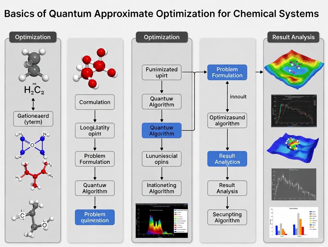
The complete QAOA process integrates the Cost and Mixer Hamiltonians into a hybrid quantum-classical feedback loop. The following diagram illustrates the logical workflow and relationships between the core components of the QAOA.

QAOA Hybrid Workflow

Experimental Protocols and Performance Analysis

Validating the performance of QAOA circuits, particularly the interplay of Cost and Mixer Hamiltonians, requires rigorous experimental protocols. These methodologies typically involve numerical simulation on classical computers, execution on real quantum processors, and comparison against classical benchmarks.

Protocol for Multi-Objective Optimization

A detailed protocol for applying QAOA to multi-objective problems, such as those relevant to chemical systems with competing objectives, is outlined below [35]:

• Problem Definition: Define m multiple objective functions. For a graph-based problem like multi-objective MAXCUT (MO-MAXCUT), this involves m different weighted graphs G_i = (V, E, w_i) sharing the same node set V and edge set E, but differing in their edge weights w_i [35].
• Parameter Training: For a smaller, representative graph (e.g., 27-node), use a classical simulator (e.g., JuliQAOA) to optimize the QAOA parameters (γ, β) for a single-objective version of the problem. A basin-hopping optimization algorithm is often used to navigate the parameter landscape [35].
• Parameter Transfer: Transfer the pre-optimized parameters to the larger target problem instance (e.g., 42-node). This leverages the finding that QAOA parameters can be transferred across problem sizes for certain problem classes, eliminating the need for costly on-device training [35].
• Circuit Execution: Execute the compiled QAOA circuit on quantum hardware. For devices with a heavy-hex topology like IBM's, the RZZ gates are compiled to native CZ gates. The minimum edge-coloring of this lattice allows all RZZ gates to be applied in three non-overlapping layers, resulting in an RZZ-depth of three per QAOA round [35].
• Solution Analysis: Approximate the Pareto front by sampling from the quantum state and identifying non-dominated solutions. Performance is evaluated using metrics like the hypervolume (HV) of the obtained solution set in the objective space, which measures the volume covered relative to a reference point [35].

Performance of QAOA Variants

Recent experimental studies have compared the performance of different QAOA implementations. The table below summarizes key quantitative findings for solving QUBO-formulated problems, such as feature selection.

Table 1: Performance Comparison of QAOA Variants on QUBO Problems [32]

Algorithm Variant	Problem Hardness (Trade-off α)	Key Performance Metric	Reported Finding	Implication for Circuit Design
Standard QAOA	Low (α closer to 0)	Time-to-Solution	Efficient for simpler problems	Standard Cost/Mixer Hamiltonians are sufficient
ADAPT-QAOA	High (α closer to 1)	Approximation Ratio & Time-to-Solution	Significantly outperforms standard QAOA	Dynamic, problem-tailored mixers improve performance on hard problems
Standard QAOA (on Superconducting qubits)	N/A	Estimated Time-to-Solution	Shorter than trapped-ion devices	Hardware platform choice impacts runtime
Standard QAOA (on Trapped-ion qubits)	N/A	Estimated Error Rates	More favorable than superconducting devices	Hardware platform choice impacts solution fidelity

Another variant, the Dynamic Adaptive Phase Operator (DAPO-QAOA, dynamically constructs the phase (cost) operator for each layer based on the output of the previous layer, rather than using a fixed Hamiltonian. Experiments on MaxCut problems show this approach can reduce the number of two-qubit RZZ gates in the circuit to about 66% of those required by standard QAOA, while also achieving a higher approximation ratio, particularly on dense graphs [33].

The Scientist's Toolkit: Essential Research Reagents

Implementing and researching QAOA circuits for chemical systems requires a suite of software and hardware "reagents." The following table details key resources mentioned across recent experimental studies.

Table 2: Key Research Tools for QAOA Circuit Implementation

Tool Name / Category	Primary Function	Relevance to Cost/Mixer Hamiltonians	Example Use Case
Qiskit (IBM) [5]	Quantum Software Development Kit	Maps high-level H_C and H_M definitions to executable quantum circuits. Provides simulators and access to real hardware.	Compiling RZZ gates to native CZ gates on IBM's heavy-hex topology [35].
JuliQAOA [35]	High-Performance QAOA Simulator	Efficiently evaluates expectation values and gradients of H_C for a given QAOA statevector. Used for classical parameter optimization.	Pre-optimizing QAOA parameters (γ, β) for a 27-node graph prior to hardware execution [35].
IBM Quantum Hardware [35] [34]	Superconducting Quantum Processor	Executes the physical quantum circuit implementing the Cost and Mixer unitaries.	Running 42-node MO-MAXCUT circuits with 3 objective functions [35].
Trapped-Ion Quantum Processor [37]	Alternative Quantum Hardware Platform	Executes QAOA circuits, often with higher fidelity two-qubit gates but potentially slower cycle times.	Demonstrating parameter fine-tuning on up to 32 qubits and 5 QAOA layers [37].
Gurobi [35]	Classical Mathematical Programming Solver	Solves Mixed Integer Programs (MIPs) to provide classical benchmarks for QAOA performance on problems like MAXCUT.	Used in the ε-constraint method to generate the Pareto front for performance comparison [35].
QuCLEAR Framework [38]	Quantum Circuit Optimizer	Reduces quantum gate count and circuit depth by classically pre-processing and simplifying circuit components.	Can be applied to optimize QAOA circuits by reducing CNOT gate count by 50.6% on average vs. Qiskit [38].

The Cost and Mixer Hamiltonians form the fundamental building blocks of the QAOA circuit, working in concert to navigate the complex landscapes of combinatorial optimization problems. While the Cost Hamiltonian (H_C) encodes the problem's objective function, the Mixer Hamiltonian (H_M) governs the exploration of the solution space. Ongoing research continues to refine these components, yielding more sophisticated mixers like the XY mixer for constrained problems and adaptive variants like ADAPT-QAOA. Experimental protocols demonstrate the feasibility of applying QAOA to multi-objective problems relevant to chemical systems, and performance analyses show that algorithm variants can significantly improve efficiency and solution quality. As quantum hardware continues to advance and algorithms become more refined, the nuanced implementation of these core Hamiltonians will be crucial for unlocking quantum advantage in chemical research and beyond.

The Quantum Approximate Optimization Algorithm (QAOA) is a hybrid quantum-classical algorithm designed to find approximate solutions to combinatorial optimization problems. In the context of chemistry, its potential is profound. Chemical problems are inherently quantum mechanical; molecules are quantum systems whose behaviors, such as molecular geometry, reaction pathways, and electronic properties, can be framed as complex optimization tasks. Classical computers struggle to simulate these systems exactly, especially when dealing with strongly correlated electrons, often relying on approximations like density functional theory [1]. QAOA, and variational quantum algorithms more broadly, offer a pathway to model these systems more accurately by leveraging the natural affinity between quantum hardware and quantum chemistry [1].

This guide details the step-by-step workflow for applying QAOA to chemical problems, framing the process within the broader thesis of developing quantum tools for chemical systems research. It is designed for researchers, scientists, and drug development professionals who seek to understand and implement this emerging methodology.

Foundational Concepts

The QAOA Framework

QAOA operates by constructing a parameterized quantum circuit whose structure is inspired by the problem to be solved. The algorithm prepares a variational quantum state by applying a sequence of two alternating operators to an initial state [39]:

• The Cost Hamiltonian (H_C): This operator encodes the problem whose ground state (lowest energy state) represents the solution. For chemistry, this typically represents the energy of a molecular system.
• The Mixer Hamiltonian (H_M): This operator drives transitions between computational basis states, facilitating exploration of the solution space. A common choice is a simple non-commuting sum of Pauli-X operations on each qubit [39].

For a circuit with p layers, the resulting variational state is: [ |\psi(\boldsymbol\gamma, \boldsymbol\beta)\rangle = \prod{k=1}^{p} e^{-i\betak HM} e^{-i\gammak HC} |+\rangle^{\otimes n} ] where (\boldsymbol\gamma = (\gamma1, \ldots, \gammap)) and (\boldsymbol\beta = (\beta1, \ldots, \betap)) are variational parameters optimized by a classical computer to minimize the expectation value of the cost Hamiltonian, (\langle \psi(\boldsymbol\gamma, \boldsymbol\beta) | HC | \psi(\boldsymbol\gamma, \boldsymbol\beta) \rangle) [40] [39].

The Hybrid Quantum-Classical Loop

The optimization of the parameters ((\boldsymbol\gamma, \boldsymbol\beta)) creates a feedback loop:

• The quantum computer prepares the state (|\psi(\boldsymbol\gamma, \boldsymbol\beta)\rangle) and measures the expectation value of (H_C).
• The classical computer uses this measurement outcome to adjust the parameters for the next iteration.
• This process repeats until the energy converges to a minimum, at which point the state (|\psi(\boldsymbol\gamma, \boldsymbol\beta)\rangle) is an approximation of the ground state of (H_C) [41].

Mapping Chemical Problems to QAOA

The first and most crucial step is to translate a chemical problem into an optimization problem compatible with QAOA.

From Electronic Structure to QUBO and HUBO

Many chemical properties are determined by the electronic structure, which involves finding the ground state energy of the system's Hamiltonian. This electronic Hamiltonian can be transformed into a qubit-representable form using techniques like the Jordan-Wigner or Bravyi-Kitaev transformation. The result is often a Hamiltonian comprising Pauli-Z operators [1].

For QAOA, this Hamiltonian serves as the cost Hamiltonian, (HC). It can be expressed in a generalized form for Higher-Order Unconstrained Binary Optimization (HUBO): [ HC = \sum J{ij} Zi Zj + \sum K{ijk} Zi Zj Z_k + \cdots ] where the terms represent interactions between two electrons (quadratic), three electrons (cubic), and higher. Recent research has successfully extended the QAOA-GPT framework to solve such HUBO problems with spin-glass Hamiltonians that include cubic interaction terms, demonstrating the algorithm's applicability beyond simple quadratic interactions [40].

Table: Key Transformations for Chemical Problems

Chemical Problem	Target Quantity	Common Cost Hamiltonian Form	QAOA Application Example
Molecular Ground State	Electronic Energy	Sum of Pauli strings (from transformed electronic Hamiltonian)	Modeling small molecules (H₂, LiH, BeH₂) [1]
Protein Folding	Free Energy of a Structure	QUBO representing atom-atom interactions and constraints	Folding of a 12-amino-acid chain on quantum hardware [1]
Reaction Pathway	Energy Barrier	HUBO mapping potential energy surface	Quantum simulation of chemical dynamics [1]

Problem Formulation Workflow

The following diagram illustrates the logical process of mapping a chemical problem onto a form suitable for a QAOA computation.

Successfully executing a QAOA experiment for chemistry requires a suite of classical and quantum resources.

Table: Essential Research Reagents and Computational Tools

Item / Resource	Category	Function / Purpose	Examples / Notes
Parameter Optimizer	Software (Classical)	Finds optimal (γ, β) parameters to minimize energy. Critical for navigating complex landscapes.	DARBO [41], Adam [41], COBYLA [41]
Quantum Simulation Framework	Software (Classical)	Models quantum circuits and computes expectation values classically for algorithm development.	PennyLane [39], Qiskit, Cirq
Graph Embedding Algorithm	Software (Classical)	Encodes topological information of problem graphs for machine-learning-enhanced QAOA.	FEATHER algorithm [40]
Quantum Processing Unit (QPU)	Hardware	Executes the parameterized quantum circuit.	Superconducting processors (e.g., IBM, Google) [41], Photonic quantum computers [42]
Cost/Mixer Hamiltonians	Algorithmic Component	Encodes the chemical problem (HC) and drives state transitions (HM).	Built-in problem sets in frameworks like PennyLane [39]
Quantum Error Mitigation (QEM)	Software/Hardware	Reduces the impact of noise on results from real quantum hardware.	Integrated QEM techniques [41]

Step-by-Step QAOA Protocol for a Chemical System

This protocol outlines the specific steps for using QAOA to find the ground state energy of a molecule, a common use case in quantum chemistry.

Experimental Workflow

The complete experimental workflow, from problem definition to result analysis, is visualized below.

Detailed Methodologies for Key Steps

• Step 2: Hamiltonian Generation: The electronic Hamiltonian in the second quantized form is generated for the specified molecule and basis set. This involves calculating one-electron and two-electron integrals using classical electronic structure packages, which are then passed to a quantum computing library.
• Step 3: Qubit Mapping: The fermionic operators of the electronic Hamiltonian are mapped to qubit (Pauli) operators. The Bravyi-Kitaev transformation is often preferred over the Jordan-Wigner transformation due to its higher efficiency for molecular simulations.
• Steps 6-7: Circuit Execution & Measurement: The quantum circuit is built by layering p sequences of the cost and mixer unitaries. The circuit is executed multiple times (shots) to estimate the expectation value (\langle H_C \rangle). This step is where noise and errors on real hardware most significantly impact results.
• Steps 8-10: Classical Optimization: The classical optimizer's role is critical. As highlighted in recent research, optimizers like Double Adaptive-Region Bayesian Optimization (DARBO) have shown superior performance for QAOA, greatly outperforming conventional optimizers in speed, accuracy, and stability, especially in the presence of noise [41]. DARBO uses a Gaussian process surrogate model and adaptive regions to efficiently navigate the complex parameter landscape.

Performance Analysis and Current Limitations

Quantitative Performance Metrics

The performance of QAOA is typically evaluated using the approximation ratio, r, which for energy problems is the ratio of the obtained energy value to the exact ground state energy (r = 1 indicates a perfect solution) [41]. The table below summarizes key findings from recent studies.

Table: QAOA Performance and Hardware Requirements

Study Focus / Molecule	System Size (Qubits)	Key Metric (Approximation Ratio)	Optimizer Used	Notes / Challenges
MAX-CUT on w3R graphs [41]	16	Approximation gap (1-r) for DARBO was 1.02-3.47x smaller than baselines	DARBO vs. Adam, COBYLA	Demonstrates DARBO's superior efficiency and stability in simulation.
Iron-Sulfur Cluster [1]	N/A	Energy estimation via hybrid algorithm	Hybrid Algorithm	Demonstrated on a qubit processor paired with a classical supercomputer.
Protein Folding (IonQ) [1]	N/A	Simulation of a 12-amino-acid chain	N/A	Largest protein-folding demonstration on quantum hardware to date.
FeMoco Simulation (Projected) [1]	~2.7 Million (physical qubits)	Required for quantum advantage	N/A	Illustrates the massive scaling required for industrially relevant problems.

Current Challenges and Outlook

Despite promising progress, applying QAOA to practical chemical problems faces significant hurdles:

• Resource Requirements: Modeling industrially relevant molecules like cytochrome P450 enzymes or the iron-molybdenum cofactor (FeMoco) for nitrogen fixation is estimated to require millions of physical qubits, far beyond current capabilities [1].
• Optimization Difficulties: The QAOA objective landscape is notorious for barren plateaus (vanishing gradients) and pervasive local minima, making parameter optimization challenging [41].
• Hardware Noise: Current NISQ devices have significant levels of noise, which disrupts computation. While error mitigation techniques exist, fault-tolerant quantum computing is needed for large-scale applications.

Ongoing research is addressing these challenges through machine learning for parameter prediction [40], improved classical optimizers like DARBO [41], and the development of more powerful and stable quantum hardware. The trajectory suggests that QAOA and other variational algorithms will play an increasingly important role in computational chemistry as the technology matures.

The Quantum Approximate Optimization Algorithm (QAOA) represents a promising framework for solving combinatorial optimization problems on noisy intermediate-scale quantum (NISQ) devices. This technical guide explores the encoding of molecular docking and protein-ligand interaction problems into the QAOA framework, providing researchers with methodologies to transform classical computational chemistry challenges into quantum-solvable formulations. We present detailed protocols for constructing cost Hamiltonians that capture the essential physics of molecular recognition, including flexible ligand docking, binding affinity prediction, and conformational selection. By bridging computational chemistry with quantum optimization, this work aims to establish a foundation for achieving quantum advantage in structure-based drug design and biomolecular simulation.

The Quantum Approximate Optimization Algorithm (QAOA) is a widely-studied method for solving combinatorial optimization problems on NISQ devices [39]. Introduced by Farhi et al., QAOA operates by constructing a parameterized quantum circuit that alternates between applying a cost Hamiltonian (encoding the problem) and a mixer Hamiltonian (facilitating state transitions) [43]. For chemical systems, this framework can be adapted to solve optimization problems related to molecular docking, protein-ligand interactions, and binding affinity prediction by carefully mapping molecular recognition physics to quantum-operable formulations.

The fundamental QAOA circuit consists of repeated applications of cost and mixer unitaries, constructing the overall unitary transformation (U(\boldsymbol\gamma, \ \boldsymbol\alpha) = e^{-i \alphan HM} e^{-i \gamman HC} \ ... \ e^{-i \alpha1 HM} e^{-i \gamma1 HC}), where (HC) is the cost Hamiltonian encoding the optimization problem, (HM) is the mixer Hamiltonian, and (\boldsymbol\gamma), (\boldsymbol\alpha) are parameters optimized classically [39]. The algorithm prepares an initial state, applies the parameterized circuit, and uses classical optimization to tune parameters until the output state yields high-quality solutions to the original problem.

For molecular docking, the "optimal solution" corresponds to the most stable binding pose and configuration, determined by physical interactions including hydrogen bonds, ionic interactions, Van der Waals forces, and hydrophobic effects [44]. The challenge lies in formulating these classical computational chemistry problems into Hamiltonians compatible with the QAOA framework while maintaining the essential physics governing molecular recognition.

Fundamentals of Molecular Docking

Molecular docking is a computational technique that predicts the preferred position and orientation of a ligand (small molecule) when bound to a protein receptor, forming a stable complex [45]. This technique stands as a pivotal element in computer-aided drug design (CADD), consistently contributing to advancements in pharmaceutical research by identifying the "best" match between two molecules based on their three-dimensional structures and chemical properties [44].

Physical Basis of Protein-Ligand Interactions

Protein-ligand interactions are governed by non-covalent binding forces that determine the stability and specificity of the resulting complex [44]. The major types of interactions include:

• Hydrogen bonds: Polar electrostatic interactions between a hydrogen atom bonded to an electronegative donor atom and another electronegative acceptor atom, with strength of approximately 5 kcal/mol [44].
• Ionic interactions: Electrostatic attractions between oppositely charged ionic pairs, highly specific but influenced by solvent effects [44].
• Van der Waals interactions: Nonspecific forces arising from transient dipoles in electron clouds when atoms approach closely, with strength of approximately 1 kcal/mol [44].
• Hydrophobic interactions: Entropically-driven associations of nonpolar molecules that exclude water from their interface [44].

The net binding affinity is quantified by the Gibbs free energy change ((\Delta G{bind})), which balances enthalpic contributions from formed bonds against entropic costs of reduced flexibility and solvent reorganization: (\Delta G{bind} = \Delta H - T\Delta S) [44].

Molecular Recognition Models

Three primary models describe the binding mechanism in molecular docking:

• Lock-and-key model: Proposes rigid complementarity between protein and ligand binding interfaces, with no conformational changes upon binding [44].
• Induced-fit model: Allows conformational changes in the protein to accommodate the ligand, resembling a "hand in glove" mechanism [44].
• Conformational selection model: Ligands selectively bind to pre-existing conformational states from an ensemble of protein structures [44].

Most modern docking approaches incorporate elements of induced-fit and conformational selection, requiring algorithms to sample both ligand orientations and protein conformational states.

Encoding Molecular Docking into QAOA Formulation

Transforming molecular docking into a QAOA-compatible problem requires mapping the physical docking problem to a cost Hamiltonian whose ground state corresponds to the optimal docking solution. This process involves discrete representation of conformational space and formulation of scoring functions as quantum-operable Hamiltonians.

Qubit Encoding Strategies

The first step in QAOA formulation establishes a correspondence between docking variables and qubit states:

Table 1: Qubit Encoding Strategies for Molecular Docking

Encoding Type	Description	Qubit Requirements	Application Context
Binary Position Encoding	Discretizes binding site into grid cells, with qubits indicating ligand atom presence in each cell	(n^3) for n×n×n grid	Rigid docking with fixed binding site
Rotation Encoding	Represents ligand orientation using Euler angles discretized into binary values	(3\log_2(k)) for k discrete angles per axis	Flexible ligand docking with rotational sampling
Conformation Encoding	Uses qubit strings to represent discrete conformational states of both ligand and protein	(m+p) for m ligand and p protein conformations	Flexible docking with side-chain mobility
Interaction Encoding	Directly encodes presence/absence of specific molecular interactions	Equal to number of potential interactions	Knowledge-based docking with known interaction patterns

Cost Hamiltonian Formulation

The cost Hamiltonian (H_C) incorporates the essential physics of molecular recognition through multiple energy terms:

[HC = H{\text{steric}} + H{\text{electrostatic}} + H{\text{H-bond}} + H{\text{hydrophobic}} + H{\text{solvation}}]

Each term can be formulated using Pauli operators acting on the encoded qubit space:

• Steric complementarity ((H_{\text{steric}})): Encourages shape matching while penalizing atomic clashes. Represented as:

  [H{\text{steric}} = \sum{i,j} V{ij} \frac{(1 - Zi)(1 - Z_j)}{4}]

  where (V{ij}) represents the steric interaction potential between atoms (i) and (j), and (Zi) is the Pauli Z operator on qubit (i) [39].

• Electrostatic interactions ((H_{\text{electrostatic}})): Models Coulombic attractions and repulsions between charged groups:

  [H{\text{electrostatic}} = \sum{i,j} \frac{qi qj}{4\pi\epsilon0 r{ij}} \frac{(1 - Zi)(1 - Zj)}{4}]

• Hydrogen bonding ((H_{\text{H-bond}})): Specific directional term that rewards proper geometry of hydrogen bond formation:

  [H{\text{H-bond}} = \sum{\text{H-bonds}} E{\text{HB}} \cdot f(\theta) \cdot \frac{(1 - Zd)(1 - Z_a)}{4}]

  where (f(\theta)) encodes angular dependence, and (Zd), (Za) correspond to donor and acceptor qubits.

• Hydrophobic interactions ((H_{\text{hydrophobic}})): Rewards clustering of nonpolar surfaces to minimize solvent exposure:

  [H{\text{hydrophobic}} = -\sum{i,j \in \text{hydrophobic}} \epsilon{hh} \frac{(1 - Zi)(1 - Z_j)}{4}]

The complete cost Hamiltonian is constructed as a weighted sum of these terms, with weights determined by their relative contributions to binding free energy.

Mixer Hamiltonian Selection

The mixer Hamiltonian (H_M) facilitates transitions between possible states while preserving constraints. For molecular docking, the standard X-axis mixer is often suitable:

[HM = \sumi X_i]

where (X_i) is the Pauli X operator on qubit (i) [39]. For problems with complex constraints, more specialized mixers may be required to maintain validity throughout the state evolution.

Experimental Protocols and Methodologies

Workflow for QAOA-Based Molecular Docking

The following diagram illustrates the complete workflow for applying QAOA to molecular docking problems:

Protocol for Minimum Viable Docking Implementation

This protocol provides a step-by-step methodology for implementing a basic QAOA-based docking system using PennyLane:

• System Preparation

  • Obtain 3D structures of protein and ligand from Protein Data Bank or predictive methods
  • Define binding site region and discretize into 2Å grid resolution
  • Identify potential hydrogen bond donors/acceptors and hydrophobic regions

• Qubit Encoding

  • Implement binary position encoding using 8×8×8 grid (512 qubits)
  • For reduced resource implementation, use coarse 4×4×4 grid (64 qubits)
  • Encode ligand rotational degrees using 3 Euler angles (10° increments)

• Hamiltonian Construction

  • Program steric complementarity term with clash penalty of 5.0 kcal/mol
  • Implement hydrogen bonding term with directional preference of 30° tolerance
  • Set hydrophobic interaction energy of -0.5 kcal/mol for contacting nonpolar atoms
  • Combine terms with weights: steric (40%), electrostatic (30%), H-bond (20%), hydrophobic (10%)

• QAOA Execution

  • Initialize with equal superposition state using Hadamard gates
  • Implement p=3 QAOA layer with alternating cost/mixer unitaries
  • Use ApproxTimeEvolution template with Trotter steps n=2 [39]
  • Measure expectation value of cost Hamiltonian

• Parameter Optimization

  • Employ gradient-based optimization with limited-memory BFGS
  • Set convergence tolerance of 10^-4 for energy changes
  • Use maximum of 1000 iterations with early stopping patience of 50

• Solution Extraction

  • Sample from final state to obtain top candidate poses
  • Decode qubit measurements to 3D coordinates and orientation
  • Refine solutions with classical molecular mechanics minimization
  • Rank by computed binding affinity and interaction complementarity

Advanced Implementation: Flexible Receptor Docking

For more realistic docking scenarios incorporating protein flexibility:

• Side-Chain Flexibility Encoding

  • Identify flexible binding site residues with conformational variability
  • Encode rotamer states for each side chain using 2-4 qubits per residue
  • Implement coordinated movement constraints to maintain protein integrity

• Extended Cost Hamiltonian

  • Add protein strain energy term to penalize unrealistic conformations
  • Include solvation energy term based on surface area exposure
  • Implement entropy penalty for excessive rigidification upon binding

• Constrained Mixer Design

  • Develop problem-specific mixer that preserves bond geometry
  • Implement swap operations between similar rotamer states
  • Use partitioned mixers for different flexibility regions

Successful implementation of QAOA for molecular docking requires both quantum software frameworks and classical computational resources.

Table 2: Essential Research Reagents and Computational Resources

Resource Category	Specific Tools/Solutions	Function/Purpose	Implementation Notes
Quantum Software Frameworks	PennyLane [39], Qiskit, Cirq	Hybrid quantum-classical algorithm development	PennyLane provides built-in QAOA templates and automatic differentiation
Molecular Visualization	PyMOL, Chimera, VMD	Structure preparation and result analysis	Critical for validating docking poses and interaction geometries
Classical Docking Software	AutoDock Vina [46], DOCK [45], Glide	Benchmarking and validation	Establish baseline performance against established methods
Force Field Parameters	AMBER, CHARMM, OPLS	Energy calculation for Hamiltonian terms	Provides physically accurate interaction potentials
Quantum Simulators	PennyLane default.qubit, Qiskit Aer	Algorithm development and debugging	Enable testing without hardware access
Quantum Hardware	IBM Quantum, IonQ, Rigetti	Experimental deployment	Current devices limited by qubit count and noise
Optimization Libraries	SciPy, NLopt	Parameter classical optimization	Gradient-based and gradient-free methods

Current Landscape and Research Directions

The field of quantum computing for chemical applications is rapidly evolving, with significant progress in hardware capabilities and algorithmic approaches. Recent industry reports indicate the quantum computing market has reached USD 1.8-3.5 billion in 2025, with projections of growth to USD 5.3 billion by 2029, reflecting strong investment in quantum technologies [20].

Hardware Advancements and Error Correction

Breakthroughs in quantum hardware are directly impacting the feasibility of complex chemical simulations:

• Google's Willow quantum chip (105 superconducting qubits) demonstrated exponential error reduction as qubit counts increased [20]
• IBM's fault-tolerant roadmap targets 200 logical qubits by 2029 capable of executing 100 million error-corrected operations [20]
• Microsoft's topological qubit architecture achieves inherent stability with reduced error correction overhead [20]
• Recent breakthroughs have pushed error rates to record lows of 0.000015% per operation [20]

These advancements are critical for molecular docking applications, which require substantial quantum resources for meaningful problem sizes.

Quantum Utility in Pharmaceutical Research

Early demonstrations of quantum utility in pharmaceutical applications show promising results:

• Google's collaboration with Boehringer Ingelheim demonstrated quantum simulation of Cytochrome P450 with greater efficiency and precision than traditional methods [20]
• IonQ and Ansys ran a medical device simulation that outperformed classical high-performance computing by 12% [20]
• Quantum algorithms for protein-ligand interaction are benefiting from co-design approaches where hardware and software are developed collaboratively [20]

Circuit Optimization Techniques

Recent developments in quantum circuit optimization directly impact the practicality of QAOA for molecular docking:

• The QuCLEAR framework reduces CNOT gate count up to 68.1% (50.6% on average) compared to standard compilers [38]
• Clifford extraction and absorption techniques move classically simulatable operations to classical post-processing [38]
• Hybrid quantum-classical circuit compilation significantly reduces quantum resource requirements [38]

These optimizations are essential for implementing molecular docking problems within current hardware constraints.

Encoding molecular docking problems into the QAOA framework represents a promising approach to leveraging quantum computing for drug discovery challenges. By carefully mapping the physical interactions governing protein-ligand recognition to cost Hamiltonians, researchers can transform classical docking problems into quantum-optimizable formulations. The methodologies presented in this guide provide a foundation for implementing such systems, from basic rigid docking to advanced flexible receptor scenarios.

As quantum hardware continues to improve in scale and fidelity, and as algorithmic approaches become more sophisticated, we anticipate increasing utility of QAOA and related quantum algorithms for molecular docking and broader computational chemistry applications. The integration of these quantum approaches with established classical methods in hybrid frameworks offers the most promising near-term path for practical impact in pharmaceutical research and development.

The Quantum Approximate Optimization Algorithm (QAOA) represents a promising hybrid classical-quantum approach for addressing complex computational challenges in drug discovery. This technical guide examines the application of QAOA to virtual screening and molecular dynamics, focusing specifically on molecular docking and conformational sampling problems. We present quantitative performance data from recent studies, detailed experimental protocols for implementing QAOA-based molecular docking, and visualization of key workflows. While current research demonstrates promising proof-of-concept results for molecular docking, evidence suggests more limited near-term applicability for protein folding problems. The integration of classical GPU acceleration with quantum algorithms emerges as a critical strategy for enhancing computational feasibility within the noisy intermediate-scale quantum (NISQ) era.

The Quantum Approximate Optimization Algorithm (QAOA) is a hybrid classical-quantum algorithm designed to produce approximate solutions for combinatorial optimization problems by leveraging quantum superposition and entanglement [43] [47]. In chemical systems research, QAOA is particularly valuable for solving NP-hard optimization problems that are computationally challenging for classical computers alone [27]. The algorithm operates by constructing a parameterized quantum circuit that alternates between a cost Hamiltonian (encoding the optimization problem) and a mixer Hamiltonian (facilitating transitions between states) [39].

For drug discovery applications, QAOA offers potential advantages in exploring complex energy landscapes and conformational spaces more efficiently than classical approaches [27] [48]. The algorithm's performance improves with increasing circuit depth parameter p, enabling better approximation of optimal solutions at the cost of greater computational resources [43]. In the NISQ era, QAOA implementations typically leverage classical hardware accelerators like GPUs to manage computational demands while compensating for current quantum hardware limitations [27].

QAOA for Molecular Docking in Virtual Screening

Problem Formulation and Mapping

Molecular docking aims to predict the optimal binding configuration between a ligand and target protein, which can be formulated as a maximum weighted clique problem on a Binding Interaction Graph (BIG) [27] [49]. In this representation:

• Nodes correspond to potential interaction pairs between protein and ligand pharmacophores
• Edges represent geometrically compatible interactions that can coexist
• Node weights reflect interaction strengths based on chemical complementarity

The molecular docking problem is mapped to a quantum optimization problem by constructing a cost Hamiltonian where the ground state corresponds to the maximum weighted clique, representing the optimal docking configuration [49]. This Hamiltonian incorporates both vertex weights (interaction strengths) and penalty terms for non-edges (incompatible interactions):

[H = \frac{1}{2}\sum{i \in V}wi(\sigma^zi - 1) + \frac{P}{4} \sum{(i,j) \notin E, i \neq j} (\sigma^zi -1)(\sigma^zj - 1)]

where (wi) are node weights, (P) is a penalty strength, and (\sigma^zi) are Pauli-Z operators [49].

Workflow Implementation

The following diagram illustrates the complete molecular docking workflow via QAOA:

Diagram 1: Molecular Docking Workflow via QAOA

DC-QAOA Technical Implementation

The Digitized-Counterdiabatic QAOA (DC-QAOA) variant enhances conventional QAOA by adding additional counterdiabatic terms that help drive the optimization toward the ground state more efficiently, potentially requiring fewer layers [27] [49]. The quantum circuit implementation includes the following key components:

Diagram 2: DC-QAOA Circuit Architecture

The DC-QAOA circuit applies parameterized quantum gates corresponding to the cost Hamiltonian, mixer Hamiltonian, and additional counterdiabatic terms (typically Pauli-Y rotations on each qubit) [49]. This approach digitizes the counterdiabatic driving phenomenon into a format executable on gate-based quantum computers.

Quantitative Performance Analysis

Molecular Docking Performance

Recent studies have evaluated QAOA performance on molecular docking problems with varying graph sizes:

Table 1: QAOA Performance on Molecular Docking Problems

Instance Size	Problem Type	Algorithm Variant	Key Performance Metrics	Reference
14-17 nodes	Molecular Docking (BIG)	DC-QAOA with warm-starting	Successfully identified binding interactions matching expected solutions; Largest published instance	[27]
12 nodes	Molecular Docking	QAOA	Previously largest published instance for molecular docking	[27]
6-8 nodes	Molecular Docking (BIG)	DC-QAOA	Implemented with penalty strength P=6-8; Demonstrated feasible execution	[49]
3-regular graphs	MaxCut (Benchmark)	QAOA (p=1)	Achieved cuts at least 0.6924 times optimal cut size	[43]

Computational Resource Requirements

The computational demands of QAOA-based approaches show distinct scaling patterns:

Table 2: Computational Resource Requirements

Resource Factor	Scaling Behavior	Implications for Molecular Applications
Circuit Depth	Grows linearly with p × number of constraints	For molecular docking, deeper circuits needed for complex binding interactions	[43]
Classical Preprocessing	Efficient for fixed p (independent of input size)	Applicable for small molecule docking with limited conformational space	[43]
GPU Acceleration	Significant speedup for simulated quantum runs	Essential for practical implementation with current hardware limitations	[27]
Parameter Optimization	Required for each problem instance	Classical optimization bottleneck for complex energy landscapes	[27] [39]

Experimental Protocols

Molecular Docking via DC-QAOA

Objective: Identify the optimal binding configuration between a ligand and protein by solving the maximum weighted clique problem on a Binding Interaction Graph (BIG) [27] [49].

Materials and Setup:

• Protein and ligand structures (experimental or modeled)
• Quantum simulation environment (e.g., NVIDIA CUDA-Q, PennyLane)
• GPU cluster for classical acceleration
• Classical optimizer (e.g., COBYLA, Adam)

Procedure:

• Pharmacore Selection: Identify key chemical functional groups governing protein-ligand interactions [49].
• Graph Construction:
  • Create Labeled Distance Graphs (LAGs) for protein and ligand
  • Generate Binding Interaction Graph (BIG) from LAGs
  • Assign node weights based on interaction complementarity
• Hamiltonian Formulation: Construct cost Hamiltonian incorporating vertex weights and non-edge penalties [49]:
  • Vertex term: (\frac{1}{2}\sum{i \in V}wi(\sigma^zi - 1))
  • Penalty term: (\frac{P}{4} \sum{(i,j) \notin E, i \neq j} (\sigma^zi -1)(\sigma^zj - 1))
• Circuit Implementation: Implement DC-QAOA circuit with parameterized cost, mixer, and counterdiabatic layers [49].
• Parameter Optimization: Execute hybrid classical-quantum optimization loop to minimize energy expectation value.
• Solution Extraction: Measure output state to identify maximum weighted clique corresponding to optimal docking configuration.

Conformational Sampling for Peptide Folding

Objective: Sample low-energy conformations of peptides using QAOA for simplified protein folding on a lattice [50].

Materials and Setup:

• Tetrahedral lattice for spatial discretization
• Simplified physical potential (e.g., Lennard-Jones)
• Quantum simulator with 20+ qubit capacity
• Random sampling comparator for performance validation

Procedure:

• Problem Encoding: Map peptide heavy atoms to lattice positions using binary variables [50].
• Hamiltonian Construction: Define cost Hamiltonian encoding Lennard-Jones potential energy.
• Circuit Optimization: Optimize QAOA parameters with depth p = 2-62 layers.
• Performance Validation:
  • Compare expected energy against known minimum
  • Evaluate sampling distribution against random guessing
  • Calculate success probability improvement over uniform sampling

The Scientist's Toolkit

Table 3: Essential Research Reagents and Computational Tools

Tool/Category	Specific Examples	Function in QAOA Experiments
Quantum Frameworks	PennyLane, CUDA-Q, Qiskit	Implement QAOA circuits, manage quantum-classical hybrid workflows	[39] [49]
Classical Accelerators	GPU Clusters, NVIDIA CUDA	Accelerate quantum circuit simulations, handle parameter optimization	[27]
Molecular Modeling	NetworkX, RDKit, Gaussian	Graph construction, molecular representation, force field calculations	[39] [48]
Optimization Methods	Warm-starting, Counterdiabatic driving	Enhance convergence, reduce quantum circuit depth requirements	[27]
Analysis Tools	Matplotlib, NumPy, Pandas	Result visualization, data processing, performance analysis	[39]

Limitations and Research Challenges

Despite promising applications, QAOA faces several significant challenges in chemical system research:

Performance Limitations: For protein folding applications, recent research indicates that QAOA requires substantial circuit depth (p > 40 layers) to achieve accurate results for simplified peptide conformational sampling [50]. In some cases, QAOA performance can be matched by random sampling with a small overhead, raising questions about its quantum advantage for certain molecular systems [50].

Resource Scaling: Computational times increase significantly with problem size, particularly for molecular docking instances beyond 12-17 nodes [27]. This scaling limitation currently restricts application to small molecular systems despite the use of GPU acceleration.

Algorithmic Challenges: The practical trainability of QAOA parameters remains difficult for complex molecular energy landscapes [50]. Barren plateaus and convergence issues present obstacles for real-world drug discovery applications where precise energy calculations are essential.

Future Outlook

Research in QAOA for chemical systems is evolving along several promising pathways. Enhanced algorithm variants like DC-QAOA and warm-start techniques show potential for improving convergence and reducing quantum resource requirements [27] [49]. Tight integration of classical molecular modeling expertise with quantum algorithm development will be essential for creating more physically realistic problem formulations [48] [50]. As quantum hardware matures, the exploration of larger molecular systems will become feasible, potentially revealing quantum advantage for specific virtual screening applications [27].

Overcoming Challenges: Practical Tips for Optimizing QAOA Performance

The advent of Noisy Intermediate-Scale Quantum (NISQ) technology represents a pivotal transition toward practical quantum computing, yet its potential is constrained by pervasive noise sources that degrade computational fidelity. Characterized by processors containing approximately 50 to 1,000 qubits without comprehensive error correction, NISQ devices operate with gate error rates typically between 10⁻³ and 10⁻² and coherence times that limit circuit depths to the order of 10²–10³ gates [51] [52]. For researchers in chemical systems and drug development, this noisy environment presents particular challenges for algorithms like the Variational Quantum Eigensolver (VQE), which aims to compute molecular ground state energies with chemical accuracy [52]. The cumulative effect of decoherence, gate infidelities, and measurement errors can obliterate the delicate quantum information needed for accurate molecular simulations, making understanding these pitfalls fundamental to extracting meaningful results from current quantum hardware.

Fundamental Types of Quantum Errors

Quantum computations on NISQ devices are affected by several distinct types of errors that jointly impact algorithmic performance:

• Phase Flip Errors (Dephasing): Result from environmental interactions that cause a qubit to lose phase coherence without energy exchange, effectively shortening the T₂ coherence time and transforming pure quantum states into statistical mixtures [53].
• Bit Flip Errors (Depolarization): Occur when qubits randomly flip their computational states (e.g., |0⟩ to |1⟩) due to thermal excitations or control imperfections, affecting both population and phase information [53].
• Gate Operation Errors: Arise from imperfect control during quantum gate implementation, particularly problematic for two-qubit gates which typically have lower fidelities (95–99%) compared to single-qubit gates (99-99.5%) [53] [52].
• Measurement Errors: Manifest during the readout process where the true quantum state is misidentified, with error rates potentially ranging from 1% to 40% depending on the hardware platform [51].

Quantitative Characterization of NISQ Hardware Performance

The table below summarizes typical error parameters across different quantum computing platforms, highlighting the challenging environment for chemical simulation algorithms:

Table 1: Representative Error Parameters for NISQ Hardware Platforms

Platform	Qubit Count	2-Qubit Gate Fidelity (%)	Typical Gate Time	Coherence Times (T₁/T₂)
IBM Eagle/Egret	27–33	99.3–99.7	~100 ns	~100 μs
Google Sycamore	72	98.6	~20 ns	~100 μs
IonQ (Trapped-Ion)	11	99.8–99.9	50–200 μs	1–10 s
Quantinuum H1	20	99.9	~100 μs	1–10 s
Pasqal (Neutral-Atom)	100	97–99	~1 ms	0.1–1 s [51]

The performance limitations of NISQ devices can be quantified through the relationship N·d·ε ≪ 1, where N is the qubit count, d is the circuit depth, and ε represents the two-qubit error rate. This inequality defines the boundary of feasible quantum computations before decoherence dominates [51]. For chemical applications using VQE, this directly constrains the complexity of molecular systems that can be accurately simulated.

Decoherence Dynamics in Quantum Simulations

The impact of noise becomes particularly pronounced in simulations of quantum dynamics. Research on lattice gauge theories under decoherence has demonstrated that gauge violation grows diffusively (∼γt) at short times due to environmental coupling at strength γ, before unitary errors eventually dominate, leading to ballistic growth (∼λ²t²) of inaccuracies [54]. For chemical system simulations, this manifests as unphysical molecular configurations and energies that deviate from experimentally verifiable values.

Experimental Protocols for Noise Characterization

Protocol 1: Randomized Benchmarking for Gate Error Rates

Objective: Characterize average gate fidelity across a quantum processor to identify operational weaknesses.

Methodology:

• Generate random sequences of Clifford gates of varying lengths (from 10 to 1000 gates)
• Each sequence concludes with an inversion Clifford that ideally returns qubits to initial state
• Execute each sequence on target NISQ hardware and measure final state fidelity
• Repeat measurements across multiple trials (typically 100-1000 shots per sequence)
• Fit the exponential decay curve: Fidelity = A·B^d + C, where d is sequence depth
• Extract average gate error: ε = (1 - B)·(n - 1)/n, where n is Hilbert space dimension

Key Metrics: Average gate fidelity, sequence fidelity decay constant, spatial error distribution across qubit topology [51]

Protocol 2: Noise Inversion for Decoherence Quantification

Objective: Quantify the decoherence effect of noise channels through physical implementability of their inverse.

Methodology:

• Prepare a set of known input states spanning the computational space
• Apply the noise channel of interest to each input state
• Characterize the output states using quantum state tomography
• Construct the Choi matrix representation Λ_ℰ of the noise channel
• Compute the physical implementability of the inverse channel: ν(ℰ⁻¹) = log₂(min Σ|qi|) where ℰ⁻¹ = Σqi𝒯i, with 𝒯i being physical quantum channels
• Establish bounds on purity reduction: -2ν(ℰ⁻¹) ≤ log₂[(𝒫(ρ)d - 1)/(𝒫(ρ₀)d - 1)] ≤ 0

Key Metrics: Physical implementability measure, purity degradation, entanglement destruction capacity [55]

Figure 1: Experimental workflow for noise characterization through physical implementability of noise inverse channels

The Scientist's Toolkit: Essential Research Reagents

Table 2: Key Experimental Resources for NISQ Noise Characterization

Resource/Technique	Primary Function	Application in Noise Studies
Randomized Benchmarking	Gate error quantification	Measures average fidelity of single and two-qubit gates
Quantum State Tomography	Full state reconstruction	Characterizes output states after noise channel application
Zero-Noise Extrapolation (ZNE)	Error mitigation	Extrapolates results to zero-noise limit by scaling noise
Dynamical Decoupling (DD)	Coherence preservation	Protects idle qubits from environmental decoherence
Twirled Readout Error Extraction (T-REx)	Measurement error mitigation	Characterizes and corrects readout errors [53]
Physical Implementability Framework	Noise strength quantification	Quantifies difficulty of simulating noise inverse operations [55]

Error Mitigation Strategies for Chemical System Simulations

Zero-Noise Extrapolation (ZNE) Protocols

Zero-Noise Extrapolation has emerged as a particularly valuable technique for chemical simulations on NISQ devices, with recent advancements improving its effectiveness:

Standard ZNE Protocol:

• Execute the target quantum circuit (e.g., VQE ansatz for molecular Hamiltonian) at native noise level
• Artificially amplify noise by specific factors (typically 1x, 2x, 3x) using pulse stretching or gate repetition
• Measure expectation values at each noise level
• Fit extrapolation function (linear, polynomial, or exponential) to the noise-scaled results
• Extract the zero-noise limit by evaluating the fit at zero noise [53] [52]

Advanced Qubit Error Probability (QEP) Extrapolation:

• Calculate individual qubit error probabilities for the target circuit using calibration data
• Execute circuit variants with intentionally amplified error rates
• Use mean QEP as the extrapolation variable rather than simple depth scaling
• Perform Richardson extrapolation to zero QEP, achieving more accurate results than standard ZNE, particularly for mid-depth circuits [56]

Experimental results demonstrate that ZNE can significantly improve computational accuracy, with one study showing enhancement of average expected result value from 0.09 to 0.35 on IBM Kyoto hardware [53].

Digital-Analog Quantum Computation (DAQC) for Enhanced Resilience

For chemical system simulations, the Digital-Analog Quantum Computation paradigm offers potential noise resilience advantages over purely digital approaches:

Implementation Workflow:

• Decompose target quantum algorithm (e.g., quantum phase estimation for molecular energies) into digital and analog blocks
• Implement single-qubit operations as digital pulses (high fidelity, fast execution)
• Execute entangling operations using the natural analog evolution of the processor's Hamiltonian
• Leverage intrinsic robustness of analog blocks to reduce susceptibility to gate errors and crosstalk
• Apply error mitigation techniques like ZNE specifically tailored to the DAQC paradigm [57]

Experimental comparisons demonstrate that DAQC consistently surpasses digital approaches in fidelity, particularly as processor size increases, achieving fidelities above 0.95 for 8-qubit computations when combined with ZNE [57].

Figure 2: Zero-noise extrapolation workflow for error mitigation in quantum computations

Machine Learning Approaches for Noise Characterization and Correction

Machine learning techniques provide adaptive solutions for noise challenges in NISQ devices:

Neural Network-Based Noise Characterization:

• Train machine learning models using final quantum state measurements as input
• Predict specific noise parameters (laser intensity fluctuation, waist, temperature, measurement error rates)
• Analyze scaling behavior with increasing qubit counts and measurement statistics
• Compare predicted parameters with independently calibrated values for validation [58]

Reinforcement Learning for Pulse Correction:

• Implement reinforcement learning framework to design optimized control pulses
• Reward functions based on reduction of measurement errors
• Generate pulses that inherently compensate for specific noise patterns in the hardware
• Deploy corrected pulses for improved algorithmic performance on neutral atoms NISQ devices [58]

Implications for Quantum Approximate Optimization in Chemical Research

For researchers applying quantum approximate optimization to chemical systems, understanding and mitigating NISQ noise is particularly critical when using algorithms like VQE for molecular energy calculations. The accumulated errors can easily exceed the threshold for chemical accuracy (1 kcal/mol), rendering computational results meaningless for drug discovery applications.

The performance of error mitigation techniques varies significantly with circuit characteristics and hardware platform. Experimental studies have demonstrated that dynamic decoupling improved average expected result values from 0.2492 to 0.3788 on IBM Osaka hardware, while T-REx showed different enhancement capabilities on IBM Kyoto systems [53]. This technique-dependent effectiveness underscores the importance of matching mitigation strategies to specific computational tasks and hardware configurations in chemical system simulations.

The fundamental limitation remains that without comprehensive error correction, NISQ devices face exponential resource scaling for achieving high-precision results in chemical computations. While current error mitigation techniques can extend the useful range of these devices, the path toward scalable quantum advantage in chemical research ultimately requires the transition to fault-tolerant quantum computing with logical qubits protected by quantum error correction codes [52].

Strategies for Parameter Optimization and Circuit Depth Management

The Quantum Approximate Optimization Algorithm (QAOA) has emerged as a prominent hybrid quantum-classical algorithm for tackling combinatorial optimization problems, a category that includes pivotal challenges in quantum chemistry such as molecular energy determination [59]. The performance and practical utility of QAOA on current Noisy Intermediate-Scale Quantum (NISQ) hardware are critically dependent on two interconnected aspects: the effective optimization of its variational parameters and the strategic management of quantum circuit depth. This guide provides an in-depth examination of advanced strategies in these domains, contextualized for researchers aiming to apply quantum optimization to chemical systems.

Parameter Optimization Strategies

Optimizing the 2p parameters (γ and β) in a QAOA circuit of depth p is a classical challenge that significantly influences the algorithm's performance. Moving beyond naive random initialization, sophisticated strategies leverage problem structure and machine learning to find good parameters efficiently.

Unsupervised Machine Learning for Parameter Setting

A powerful approach to reduce the number of costly quantum circuit evaluations involves using unsupervised machine learning to infer good initial parameters based on previously solved problem instances [60].

• Methodology: The process begins by generating a training dataset composed of many problem instances (e.g., molecular fragments or particular graph topologies) and their corresponding optimal QAOA parameters. This dataset is then used to train a model in an unsupervised manner. Strategies include:
  • Clustering on Angle Values: Directly clustering the optimized parameter values (γ, β) themselves.
  • Clustering on Instance Features: Using descriptive features of the problem instance (e.g., graph diameter, degree distribution for molecular connectivity) as input for clustering.
  • Variational Graph Autoencoders: Employing a graph neural network to generate a compressed latent representation of the problem instance, which is then used for clustering.
• Protocol: For a new, unseen problem instance, its features or graph encoding are computed. The model then assigns it to a pre-existing cluster. The representative parameters (e.g., centroid angles) of that cluster are used directly as the QAOA parameters for the new instance, bypassing the classical optimization loop entirely [60].
• Application Note: This strategy is exceptionally valuable in recursive or divide-and-conquer algorithms where QAOA is a subroutine, and the number of quantum circuit calls must be minimized. Research has shown this can achieve median approximation ratios of 0.94 for standard problems while drastically reducing circuit calls [60].

Meta-Learning and Parameter Transfer

The empirical observation that optimal QAOA parameters tend to concentrate for instances from similar distributions enables transfer learning strategies [60].

• Meta-Learning Protocol: A meta-learner, often a simple neural network, is trained to predict good initial QAOA parameters. The input to the network can be meta-features of the QAOA circuit or the problem instance. The trained model provides a smart initialization for a classical optimizer, significantly reducing the number of optimization iterations required to find a good solution [60].
• Layerwise Parameter Transfer: This strategy is fundamental for managing depth. The optimal parameters found for a QAOA circuit at depth p are used to initialize the optimizer for depth p+1. Typically, the new parameters are initialized as (γ₁, γ₂, ..., γₚ, γₚ), and (β₁, β₂, ..., βₚ, βₚ), and then fine-tuned [61] [60].

Bayesian Optimization for Parameter Initialization

For complex problems where parameters do not readily concentrate, Bayesian optimization offers a robust strategy for initializing large-scale QAOA problems.

• Methodology: This protocol involves first solving a set of smaller, tractable problem instances (either in terms of qubit count or classical simulability). A Bayesian optimization model is then trained on the parameters and performance from these small-scale instances.
• Experimental Protocol: The trained Bayesian model is used to surrogate the parameter landscape of the large-scale target problem. It intelligently proposes new parameter sets to evaluate on the quantum hardware, balancing exploration and exploitation to find high-performance parameters with fewer quantum device calls [62].

Table 1: Comparison of Parameter Optimization Strategies

Strategy	Core Principle	Key Advantage	Best-Suited For
Unsupervised ML (Clustering)	Infers parameters from instance similarity [60]	Drastically reduces quantum circuit calls; no optimization loop	Recursive algorithms; distributions of similar instances
Meta-Learning	Neural network predicts initial parameters [60]	Provides high-quality starting points for optimizers	Problems with readily available meta-features
Parameter Transfer	Parameters from depth p warm-start depth p+1 [61]	Accelerates convergence for deeper circuits	Progressive circuit depth expansion
Bayesian Optimization	Surrogate model navigates parameter landscape [62]	Efficient parameter finding for complex landscapes; robust to noise	Large-scale problems and noisy hardware

Figure 1: Unsupervised and Meta-Learning Parameter Workflow. This diagram illustrates the process of using classical machine learning to predict QAOA parameters, minimizing calls to the quantum processor.

Circuit Depth Management Strategies

Circuit depth is a primary determinant of feasibility on NISQ devices. Deeper circuits offer theoretically better performance but are more susceptible to noise. Effective depth management is therefore crucial.

Dynamic Depth QAOA (DDQAOA)

The DDQAOA framework directly addresses the challenge of pre-selecting a fixed depth p by allowing the circuit to grow adaptively [61].

• Experimental Protocol:
  • Initialization: Begin optimization at a shallow depth, typically p=1.
  • Optimization & Evaluation: Optimize the parameters for the current depth p and evaluate the solution quality (e.g., using the approximation ratio).
  • Convergence Check: If the solution quality has not improved beyond a predefined threshold, increment the depth to p+1.
  • Warm-Start: Transfer the optimized parameters from depth p to initialize the first p layers at depth p+1, as described in Section 2.2.
  • Termination: Repeat steps 2-4 until a maximum depth is reached or the solution quality converges.
• Performance: Testing on combinatorial problems has shown that DDQAOA can achieve results comparable to standard fixed-depth QAOA but with significantly fewer quantum resources. For example, it used 217% fewer CNOT gates for a 10-qubit problem compared to a fixed p=15 QAOA while delivering a superior approximation ratio [61].

Circuit Compilation and Optimization

Reducing the physical gate count of a QAOA circuit of a given depth p is equivalent to making it shallower and more noise-resilient.

• QuCLEAR Framework Protocol: This is a classical pre-processing technique for quantum circuits [38].
  • Clifford Extraction: Identify and move all Clifford gates—a class of gates that can be efficiently simulated on a classical computer—to the end of the circuit.
  • Clifford Absorption: These rearranged Clifford operations are then handled by classical post-processing of the measurement results, rather than being executed on the quantum hardware.
• Outcome: This method has demonstrated an average reduction of 50.6% in the number of two-qubit (CNOT) gates for benchmarks including QAOA, directly translating to shorter circuit depth and execution time [38].

Low-Depth Algorithmic Variants

Research is exploring algorithm variants that achieve high performance at minimal depth.

• Instantaneous Quantum Polynomial (IQP) Circuits: One approach uses a parameterized IQP circuit with the same depth as 1-layer QAOA but incorporates additional corrections. The parameters for this circuit can be efficiently trained on a classical computer, avoiding the training issues of deeper QAOA circuits. This method has been shown to amplify the probability of finding the optimal solution compared to standard 1-layer QAOA [14].

Table 2: Comparison of Circuit Depth Management Strategies

Strategy	Core Principle	Key Advantage	Reported Efficacy
Dynamic Depth (DDQAOA)	Adaptively increases depth p based on convergence [61]	Avoids over-/under-parameterization; saves quantum resources	217% fewer CNOT gates (10-qubit) vs fixed p=15 [61]
Circuit Optimization (QuCLEAR)	Classically absorbs Clifford gates from the circuit [38]	Reduces gate count and depth without changing algorithm	50.6% avg. reduction in CNOT gates [38]
Low-Depth Variants (IQP)	Uses a differently structured, classically-trainable low-depth circuit [14]	Mitigates noise; avoids barren plateaus in training	2^0.23n runtime enhancement over 1-layer QAOA [14]

Figure 2: Dynamic Depth QAOA (DDQAOA) Flowchart. This diagram outlines the adaptive process of starting with a shallow circuit and incrementally increasing its depth until performance converges.

Application to Chemical Systems Research

The application of QAOA in quantum chemistry, such as finding the ground state energy of molecules, is a primary target. The strategies discussed above are directly relevant in this context.

Case Study: The [4Fe-4S] Molecular Cluster

A recent hybrid quantum-classical study on the [4Fe-4S] cluster, a complex biologically relevant molecule, provides a template for application [59].

• Objective: Determine the electronic ground state (lowest energy level) of the [4Fe-4S] cluster by solving for its wave function.
• Challenge: The Hamiltonian matrix for this system is enormous, and classical heuristics for pruning it to a manageable size are not always reliable.
• Hybrid Protocol:
  • Quantum Pre-processing: A quantum computer (an IBM Heron processor) was used to analyze the full Hamiltonian and identify the most important components, replacing classical heuristics with a more rigorous quantum-based selection [59].
  • Classical Post-processing: The pruned, relevant part of the Hamiltonian was then fed into a high-performance classical supercomputer (RIKEN's Fugaku) to solve for the exact wave function [59].
• Connection to QAOA: While this specific study did not use QAOA, the paradigm is directly analogous. The quantum processor's role is to handle the part of the problem that is intractable for classical computers—in this case, identifying important parts of the Hamiltonian, a task that could be framed as an optimization problem. The parameter and depth strategies from previous sections are critical for making the quantum part of such a hybrid workflow efficient and accurate on NISQ hardware.

The Scientist's Toolkit: Essential Research Reagents

Table 3: Key "Reagents" for Quantum Chemistry Optimization Experiments

Item / Resource	Function / Role in the Experiment
Hybrid Quantum-Classical Compute Stack	Provides the physical hardware for algorithm execution; quantum processor for state preparation/ansatz, classical computer for optimization/analysis [59].
Molecular Hamiltonian	The mathematical description of the energy of the quantum chemical system; encoded into the QAOA cost Hamiltonian, H_C [59].
Problem Encoding (QUBO/Ising)	A formalism for translating the molecular energy minimization problem into a binary optimization problem suitable for QAOA [5] [60].
Classical Optimizer	A classical algorithm (e.g., COBYLA, SPSA) that adjusts QAOA parameters (γ, β) to minimize the energy expectation value ⟨H_C⟩ [60].
Circuit Compiler (e.g., QuCLEAR, Qiskit)	Software that translates a high-level QAOA circuit into a hardware-specific gate sequence and applies optimizations to reduce gate count and depth [38].
Parameter Initialization Strategy	The method (e.g., unsupervised learning, meta-learning, interpolation) used to select the starting point for the classical optimizer [60].

The practical application of the Quantum Approximate Optimization Algorithm to consequential problems in chemical systems research hinges on the effective management of its parameters and circuit depth. Strategies such as unsupervised machine learning for parameter prediction, dynamic and adaptive control of circuit depth, and classical compilation techniques for circuit compression are not isolated improvements but are synergistic. When combined within a hybrid quantum-classical computing paradigm, they form a robust methodology that maximizes the use of limited quantum resources. This approach allows researchers to begin extracting tangible value from NISQ-era devices for exploring complex molecular systems, paving the way for more advanced applications as quantum hardware continues to evolve.

Error Mitigation Techniques and Hardware Advancements

Quantum computing holds transformative potential for chemical systems research, particularly in simulating molecular structures and reactions with a precision that is computationally infeasible for classical computers [63]. However, the current era of Noisy Intermediate-Scale Quantum (NISQ) devices is characterized by high error rates that impede reliable computation [64]. For researchers leveraging the Quantum Approximate Optimization Algorithm (QAOA) and similar variational methods for chemical problems, managing these errors is a prerequisite for obtaining meaningful results. This guide synthesizes the latest advancements in quantum error mitigation techniques and the hardware improvements that make them viable, providing a practical framework for their application in chemical research.

Foundational Error Management Concepts

Before delving into specific techniques, it is crucial to understand the taxonomy of quantum error reduction. These strategies are not mutually exclusive and are often deployed in concert to maximize the fidelity of results from contemporary quantum processors.

• Error Suppression: This is a proactive technique that leverages flexibility in quantum platform programming to execute a circuit correctly given anticipated hardware imperfections. It operates by either avoiding errors (e.g., via intelligent circuit routing) or actively suppressing them through physical principles like coherent averaging. It is deterministic, providing error reduction in a single execution without the need for repeated runs or statistical averaging. It is highly effective against coherent errors but cannot address inherent random errors like qubit decoherence (T1 processes) [65].

• Error Mitigation: This is a reactive set of techniques that address noise in post-processing. They do not prevent errors from occurring but rather reduce their average impact on the output by performing many repetitions of the target circuit and classically post-processing the noisy outputs. Common methods include Zero-Noise Extrapolation (ZNE) and Probabilistic Error Cancellation (PEC). A key limitation is that they are generally not applicable for preserving full output distributions, a requirement for many sampling algorithms. Furthermore, they often incur a significant, sometimes exponential, overhead in the number of circuit executions required [65].

• Quantum Error Correction (QEC): QEC is an algorithmic approach designed to deliver fault tolerance by encoding logical quantum information across many physical qubits. This redundancy allows errors to be identified and corrected on the fly. While foundational for large-scale quantum computing, QEC is currently resource-intensive. Recent demonstrations, such as Google's, used 105 physical qubits to realize a single logical qubit, drastically reducing the number of qubits available for the core algorithm. Practical, scalable QEC use remains a future goal, though rapid progress is being made [65].

Table 1: Core Quantum Error Reduction Strategies

Strategy	Operational Principle	Key Advantage	Primary Limitation	Best Suited For
Error Suppression	Proactive avoidance & cancellation via pulse-level control & compilation.	Deterministic; no sampling overhead.	Cannot correct inherent stochastic (incoherent) errors.	All applications, as a first line of defense.
Error Mitigation	Reactive post-processing of results from many noisy circuit executions.	Can address both coherent and incoherent errors.	Exponential sampling overhead; not for full distribution tasks.	Estimation tasks (e.g., energy calculation in VQE).
Error Correction	Algorithmic encoding of logical information into many physical qubits.	Provides a path to fault tolerance; can handle arbitrary errors.	Massive qubit overhead and slower logical operations.	Long-term, large-scale fault-tolerant computation.

Advanced Error Mitigation Techniques for Chemical Systems

For chemical applications like ground state energy calculation, where the output is an expectation value, error mitigation techniques are particularly valuable. The following methods have been specifically developed or adapted for the complex wavefunctions encountered in chemical simulations.

Multireference-State Error Mitigation (MREM)

Background and Motivation: The previously established Reference-state Error Mitigation (REM) is a cost-effective method that calibrates out hardware noise using a classically tractable reference state, such as the Hartree-Fock state [64]. However, its effectiveness is limited for strongly correlated systems (e.g., bond breaking, transition metal complexes), where the true wavefunction is a multireference state—a linear combination of multiple Slater determinants with similar weights. In these cases, a single determinant does not provide sufficient overlap with the true ground state, leading to inaccurate error mitigation [64].

Methodology: MREM extends the REM framework to systematically incorporate multireference states [64].

• State Selection: An approximate multireference wavefunction is generated using an inexpensive classical method (e.g., CASSCF, DMRG). This wavefunction is truncated to include only a few dominant Slater determinants to balance expressivity and noise sensitivity.
• State Preparation: The selected multireference state is prepared on the quantum hardware using a circuit composed of Givens rotations. These rotations provide a structured, symmetry-preserving (particle number, spin) method to build linear combinations of Slater determinants from an initial reference configuration.
• Error Calibration: The energy of this multireference state is calculated exactly on a classical computer. The state is then prepared and measured on the quantum device to quantify the hardware-induced energy error.
• Mitigation: The error profile learned from the multireference state is used to mitigate the energy error of the target, correlated ground state obtained from a VQE calculation, under the assumption that noise affects both states similarly.

Experimental Workflow: The following diagram illustrates the MREM protocol for a strongly correlated molecule.

Error Mitigation for Partially Error-Corrected Computers

Emerging Hybrid Paradigm: A frontier in error management involves hybrid systems containing both logical (error-corrected) and physical (noisy) qubits. A recent theoretical study proposes a method that uses logical ancilla qubits to drastically reduce the sampling complexity of error cancellation techniques like PEC [66].

Methodology and Trade-off: In this approach, logical qubits are used as reliable resources to implement "convex combinations of channels," which is central to PEC. The result is a potential continuous trade-off space: using more logical resources can arbitrarily reduce the sampling overhead, in the limiting case achieving a sampling complexity of O(1), which circumvents known exponential lower bounds for other mitigation techniques [66]. However, this comes at the cost of an exponential increase in circuit depth, leading to a conjecture that any error mitigation protocol with (sub-)polynomial sample complexity requires exponential time and/or space, even when logical qubits are utilized [66].

Key Hardware Advances Enabling Error Mitigation

The efficacy of the techniques described above is inextricably linked to progress in quantum hardware. Breakthroughs in 2024-2025 have created a more robust foundation for deploying error mitigation in chemical research.

Breakthroughs in Qubit Performance and Error Correction

Hardware platforms across different modalities have demonstrated significantly improved performance, crossing critical thresholds for error correction and mitigation.

• Google's Willow Chip: This 105-qubit superconducting processor features best-in-class performance with single-qubit gate fidelities of 99.97%, entangling gate fidelities of 99.88%, and readout fidelity of 99.5%, operating at nanosecond speeds. Most significantly, it demonstrated "below-threshold" operation for a quantum error-correcting code, where increasing the number of qubits in the code reduces the overall logical error rate—a fundamental requirement for scalable fault tolerance [20] [67].

• Advanced Qubit Architectures: Companies are developing novel qubit designs to inherently reduce error rates. Alice & Bob's cat qubits are a prominent example, leveraging a novel superconducting circuit design to suppress bit-flip errors. This allows for a more efficient error correction code focused only on phase-flips. The company estimates this can reduce the physical qubit requirements for simulating complex molecules like the nitrogen-fixing FeMoco and the drug-metabolizing Cytochrome P450 by 27-fold (from 2.7 million to 99,000 qubits) compared to previous estimates, dramatically shortening the timeline for practical quantum chemistry [68].

• Diverse Platform Progress: Trapped-ion systems have achieved two-qubit gate fidelities above 99.9%, while neutral-atom platforms have demonstrated early forms of logical qubits. Microsoft, in collaboration with Atom Computing, demonstrated 28 logical qubits encoded onto 112 atoms [20].

Table 2: 2024-2025 Hardware Performance and Error Correction Milestones

Company/Institution	Platform	Key Milestone	Reported Error Rates / Performance	Implication for Error Mitigation
Google [20] [67]	Superconducting	Willow processor; below-threshold QEC.	Gate fidelities >99.88%; exponential error reduction with qubit count.	Reduces the baseline error rate that mitigation must address; validates path to FTQC.
Alice & Bob [68]	Superconducting (Cat Qubits)	Intrinsic bit-flip suppression.	27x reduction in physical qubits needed for FeMoco simulation.	Lowers the resource barrier for meaningful quantum advantage in chemistry.
IonQ [20]	Trapped Ion	Outperformed classical HPC in a medical device simulation.	36-qubit system showed 12% speedup.	Provides a tangible, early case of utility for chemically-relevant problems.
Microsoft & Atom Computing [20]	Neutral Atom	High-count logical qubit entanglement.	28 logical qubits encoded onto 112 atoms; 24 logical qubits entangled.	Demonstrates scaling of logical encoding, a core requirement for FTQC.

Classical Co-Processing and Circuit Optimization

The "full-stack" nature of quantum computing means that classical processing is a critical component of error management.

• The Decoding Bottleneck: Real-time quantum error correction has been identified as the industry's defining engineering challenge. The classical electronics must process millions of error signals per second and feed back corrections within about one microsecond, a data rate comparable to processing a global video streaming platform every second [69]. Advances in specialized decoding hardware are essential to unlock QEC.

• Circuit Optimization Frameworks: Classical tools can dramatically reduce the noise a quantum circuit is exposed to by minimizing its gate count. The QuCLEAR framework, for example, converts a quantum circuit into a smaller hybrid quantum-classical circuit by identifying and extracting "Clifford" subcircuits that can be efficiently simulated on a classical computer. This approach has been shown to reduce the number of two-qubit (CNOT) gates by up to 68.1% on average, directly lowering the circuit's vulnerability to errors without any quantum hardware changes [38].

A Practical Guide for Chemical Researchers

Selecting the right error management strategy is contingent on the specific characteristics of the chemical problem and the available quantum resources.

Strategic Selection of Error Reduction Techniques

The following decision workflow provides a guided path for researchers to select appropriate error reduction strategies based on their application's requirements.

The Scientist's Toolkit: Essential Research Reagents

For experimental quantum chemists, the following software tools and theoretical constructs are essential "reagents" for implementing the discussed error mitigation techniques.

Table 3: Essential Reagents for Quantum Error Mitigation Experiments

Reagent / Tool	Type	Primary Function in Error Mitigation	Application Note
Givens Rotation Circuits [64]	Quantum Circuit Component	Efficiently prepares multireference states as linear combinations of Slater determinants.	Preserves particle number and spin symmetry; crucial for MREM.
Clifford Circuit Simulator [38]	Classical Software	Identifies and classically simulates portions of a quantum circuit (as in QuCLEAR).	Reduces quantum circuit depth and gate count, minimizing exposure to noise.
Variational Quantum Eigensolver (VQE) [64]	Hybrid Algorithm	Serves as the primary framework for computing ground state energies on NISQ devices.	The host algorithm for which REM and MREM are applied.
Hartree-Fock State [64]	Classical Wavefunction	Serves as the initial state and reference for single-reference REM in weakly correlated systems.	Classically trivial to compute; easy to prepare on a quantum computer.
Multireference State (e.g., from CASSCF) [64]	Classical Wavefunction	Provides a high-overlap reference state for strongly correlated systems in MREM.	Must be truncated to a few determinants to balance accuracy and noise.

The path to quantum advantage in chemical systems research is being paved by simultaneous innovations in error-aware algorithms and more resilient hardware. Error mitigation techniques like MREM are expanding the class of tractable molecular problems, especially for strongly correlated systems crucial in drug discovery and catalyst design. Meanwhile, hardware advances in qubit fidelities, novel architectures like cat qubits, and the first demonstrations of practical error correction are steadily raising the ceiling of what is possible. For the research scientist, a strategic approach that combines robust error suppression, chemically intelligent mitigation like MREM, and a clear-eyed view of the evolving hardware landscape is essential for extracting maximum value from today's quantum computers and preparing for the fault-tolerant machines of tomorrow.

Hybrid Quantum-Classical Approaches for Robust Results

The integration of quantum computing with classical machine learning architectures presents a transformative opportunity for computational chemistry and drug discovery. This technical guide explores hybrid quantum-classical approaches that leverage parameterized quantum circuits as compact, expressive components within larger classical frameworks. These architectures are demonstrating significant improvements in accuracy, privacy, and computational efficiency, offering a practical path toward quantum advantage in simulating complex chemical systems. By bypassing fundamental limitations like the measurement bottleneck and enhancing robustness in molecular simulations, hybrid models enable researchers to tackle quantum chemistry problems that remain intractable for purely classical methods. This document provides experimental protocols, performance analyses, and implementation guidelines to equip researchers with the tools needed to deploy these advanced computational techniques in chemical systems research.

Hybrid quantum-classical architectures represent the most viable near-term approach to harnessing quantum computational power for chemical systems research. Unlike pure quantum computing, which requires fault-tolerant hardware not yet available, hybrid models integrate parameterized quantum circuits as functional blocks within classical neural networks or optimization algorithms. This integration creates systems that can learn more effectively from smaller datasets, reduce edge-case errors, and maintain stronger performance on complex molecular simulations – critical advantages in drug discovery and materials science where experimental data is often limited and computational demands are extreme.

The fundamental premise underlying these approaches is that quantum circuits can perform specific transformations that classical systems cannot efficiently replicate, particularly when dealing with highly correlated quantum systems. In chemical research, this capability is invaluable for simulating electronic structures, molecular dynamics, and reaction pathways where classical computational methods face exponential scaling limitations. Research indicates hybrid models achieve up to 55% accuracy improvement over quantum baselines while maintaining enhanced privacy protections and reducing parameter counts by 10-20% compared to classical models [70]. These improvements occur because quantum components can create more compact and expressive representations of molecular wavefunctions and potential energy surfaces.

Core Architectural Principles

Overcoming the Measurement Bottleneck

A fundamental limitation in quantum machine learning is the measurement bottleneck, where high-dimensional classical inputs are compressed into a smaller number of quantum observables, restricting information transfer and compromising model performance. Innovative hybrid architectures address this through residual bypass connections that combine processed quantum features with original raw input data before classification [70]. This approach preserves information that would otherwise be lost during quantum measurement, enhancing both accuracy and privacy without increasing quantum circuit complexity.

The residual hybrid architecture operates through a structured workflow:

• Classical Encoding: Classical input data (molecular descriptors, structural parameters) are encoded into quantum states using feature mapping techniques
• Quantum Transformation: Parameterized quantum circuits process these states to generate quantum features
• Residual Connection: Original classical inputs bypass the quantum system and combine with quantum features
• Classical Processing: A projection layer reduces dimensionality before final classification or regression

This architecture has demonstrated particular effectiveness in federated learning environments for chemical research, where data privacy is paramount. By transmitting only hybrid features rather than raw molecular data, researchers can collaborate across institutions while protecting sensitive compound information [70].

Strategic Placement of Quantum Components

The performance gains of hybrid models depend critically on the strategic placement of quantum components within classical architectures. Research identifies several effective integration patterns, each optimized for specific chemical applications:

• Quantum Head (Q-Head): Placing a quantum block immediately before the final decision layer in convolutional neural networks, ideal when features are strong but decision boundaries show instability in molecular property prediction [71]
• Quantum Feature Map: Positioning quantum circuits at the model front-end to transform pre-reduced molecular descriptors (e.g., PCA-transformed quantum chemical features) before further classical processing [71]
• Quantum-Modulated Gates: Integrating small quantum blocks within recurrent architectures to modulate update mechanisms, beneficial for temporal chemical processes like reaction kinetics [71]

These integration patterns function as "flavor enhancers" rather than complete replacements for classical components, adding unique capabilities without requiring system overhaul [71]. The optimal approach maintains small, shallow quantum circuits rather than deep, complex ones, as simpler circuits demonstrate better trainability and noise resilience on current hardware.

Table 1: Quantum Integration Patterns for Chemical Applications

Integration Pattern	Optimal Use Case	Key Advantage	Chemical Application Example
Quantum Head (Q-Head)	Strong features with unstable decision boundaries	Improves calibration, reduces edge-case errors	Molecular property prediction
Quantum Feature Map	Pre-reduced molecular descriptors	Enhances geometric separation in feature space	Quantum chemical descriptor transformation
Quantum Pooling	Preserving subtle structural patterns	Retains nuanced information while reducing dimensionality	Molecular graph convolution networks
Quantum-Modulated Gate	Temporal chemical processes	Captures long-range dependencies in sequence data	Reaction kinetics prediction

Experimental Methodologies & Protocols

Residual Hybrid Model Implementation

Implementing a residual hybrid model for chemical systems requires careful attention to the interface between quantum and classical components. The following protocol details the methodology for constructing and training such models:

Quantum Circuit Configuration:

• Employ parameterized quantum circuits with 8-16 qubits for initial experiments
• Utilize entangling layers followed by parameterized single-qubit rotations
• Implement amplitude or angle encoding for classical-to-qubit transformation
• Set circuit depth between 3-10 layers to balance expressivity and trainability

Training Methodology:

• Initialize both classical and quantum parameters using Xavier/Glorot initialization
• Employ hybrid backpropagation with automatic differentiation for classical parameters
• Utilize parameter-shift rules for quantum circuit gradients
• Implement mini-batch training with batch sizes of 32-128 depending on dataset size
• Use Adam optimizer with learning rate 0.001-0.01, adjusted based on validation performance

Residual Connection Implementation:

• Maintain original input dimensions before combining with quantum features
• Implement projection layers to reduce combined feature dimensionality before classification
• Apply batch normalization to stabilize training across quantum and classical pathways
• Use skip connections to ensure gradient flow through both pathways

Experiments across multiple chemical datasets demonstrate these models achieve comparable accuracy to classical models with 10-20% fewer parameters while providing enhanced privacy guarantees [70]. The residual connection specifically addresses the measurement bottleneck by preserving information that would otherwise be lost during quantum state measurement.

Chemical System Simulation Protocol

Quantum simulation of chemical systems requires specialized approaches tailored to molecular complexity. The following protocol, adapted from Quantum Systems Accelerator research, details methodology for simulating molecular systems:

System Preparation:

• Select target molecule and identify key quantum properties for simulation (e.g., electronic structure, spin interactions)
• Prepare molecular Hamiltonian using Hartree-Fock or DFT approximations as starting point
• Map electronic structure to qubit representation using Jordan-Wigner or Bravyi-Kitaev transformations
• Determine optimal qubit count and circuit depth based on molecular complexity

Quantum Circuit Design:

• Implement Variational Quantum Eigensolver (VQE) or Quantum Approximate Optimization Algorithm (QAOA) circuits
• Design ansatz architecture specific to molecular symmetry and properties
• Incorporate hardware-efficient gates when targeting specific quantum processors
• Apply error mitigation techniques tailored to device characteristics

Execution and Measurement:

• Execute circuits using shot-based sampling (typically 1,000-10,000 shots per measurement)
• Employ measurement reduction techniques (e.g., qubit-wise commuting groups) to minimize resource requirements
• Implement iterative parameter optimization using classical co-processors
• Apply readout error mitigation through calibration data

This approach has successfully simulated systems including zero-field NMR spectra of acetonitrile's methyl group using only 4 qubits, demonstrating practical application of near-term quantum devices to chemical analysis [72]. The methodology enables accurate determination of molecular properties that are challenging for classical computation alone.

Diagram 1: Chemical System Simulation Workflow

Optimization Algorithm Implementation

For combinatorial optimization problems in chemical research (such as molecular conformation analysis or protein folding), specialized quantum-enhanced algorithms demonstrate significant performance improvements. The following protocol details implementation of the Instantaneous Quantum Polynomial (IQP) optimization approach:

Algorithm Configuration:

• Initialize parameters using classical approximations or warm-start techniques
• Design IQP circuit architecture with all-to-all connectivity when possible
• Set circuit depth equivalent to 1-layer QAOA for resource efficiency
• Configure parameter training on classical computers to avoid quantum resource depletion

Execution Parameters:

• Employ 20.32n shots for n binary variables in the optimization problem
• Implement progressive shot allocation based on problem difficulty
• Utilize classical post-processing to identify optimal solutions from measurement samples
• Apply solution verification through classical methods when possible

Experimental results on Quantinuum's H2 quantum computer demonstrate this algorithm successfully solved 136 of 312 problem instances optimally, including a 30-qubit instance that required identifying the unique optimal solution among >1 billion candidates [14]. This represents a significant advancement in applying quantum resources to complex optimization problems in chemical systems.

Performance Analysis & Benchmarking

Quantitative Performance Metrics

Rigorous evaluation of hybrid quantum-classical models requires comparison against classical baselines across multiple dimensions. Research demonstrates consistent advantages for hybrid approaches in chemical-relevant tasks:

Table 2: Hybrid vs. Classical Model Performance Comparison

Metric	Pure Classical	Hybrid Quantum-Classical	Improvement
Validation Accuracy	98.21% (MNIST), 32.25% (CIFAR100), 63.76% (STL10)	99.38%, 41.69%, 74.05%	+1.17%, +9.44%, +10.29%
Training Time/Epoch	108.44s (MNIST)	21.23s (MNIST)	5.1x faster
Parameter Efficiency	Baseline	6-32% fewer parameters	More efficient representation
Adversarial Robustness	10.80% (MNIST)	45.27% (MNIST)	4.2x more robust
Privacy Robustness	High privacy leakage	Significantly stronger guarantees	Enhanced data protection

The performance advantages are most pronounced on complex datasets, with hybrid models achieving up to 10.29% higher accuracy on challenging vision tasks that mirror the complexity of molecular pattern recognition [73]. Additionally, hybrid models demonstrate 5-12x faster training times and superior parameter efficiency, creating more compact models that maintain high performance [73].

Chemical Application Performance

In domain-specific chemical applications, hybrid approaches demonstrate compelling advantages:

Molecular Simulation:

• Quantum simulation of NMR spectra enables structural determination of molecules like acetonitrile using only 4 qubits [72]
• Compressed sensing techniques reduce resource requirements while maintaining accuracy in quantum dynamics simulation
• Rydberg atom arrays provide flexible toolbox for simulating strongly correlated quantum systems in transition metal compounds [72]

Drug Discovery Applications:

• Google's collaboration with Boehringer Ingelheim demonstrated quantum simulation of Cytochrome P450 with greater efficiency and precision than traditional methods [20]
• Quantum resource requirements have declined sharply while hardware capabilities improve, positioning quantum systems to address Department of Energy scientific workloads within 5-10 years [20]
• The ADAPT-GQE framework achieved a 234x speed-up in generating training data for complex molecules like imipramine, crucial to pharmaceutical development [14]

These applications demonstrate the growing practical utility of hybrid quantum-classical approaches for real-world chemical and pharmaceutical challenges, particularly in scenarios where classical methods face fundamental computational barriers.

Research Reagent Solutions

Implementing hybrid quantum-classical experiments requires both computational and physical resources. The following table details essential components for constructing effective research pipelines:

Table 3: Essential Research Reagents & Computational Resources

Resource Category	Specific Solutions	Function & Application
Quantum Hardware Platforms	Quantinuum H-Series, IBM Quantum Systems, Atom Computing Neutral Atoms	Provide physical qubits for circuit execution; vary in qubit count, connectivity, and fidelity
Quantum Software Tools	NVIDIA CUDA-Q, Quantinuum's Guppy, Qiskit, PennyLane	Enable hybrid algorithm development, quantum-classical integration, and circuit optimization
Classical Co-Processing	NVIDIA Grace Blackwell, GPU Clusters, High-Performance Computing	Accelerate classical components, parameter optimization, and error correction decoding
Chemical Simulation Packages	Quantinuum's InQuanto, QSimulate, NVIDIA CUDA-QX	Provide domain-specific tools for molecular Hamiltonian preparation and chemical property calculation
Error Mitigation Tools	Readout Error Mitigation, Zero-Noise Extrapolation, Probabilistic Error Cancellation	Improve result accuracy without physical error correction, essential for near-term devices
Hybrid Algorithm Libraries	QAOA, VQE, IQP Circuits, TensorFlow Quantum	Pre-built implementations of hybrid algorithms for optimization and eigenproblem solving

The integration across these resources creates the foundation for effective hybrid quantum-classical research. Notably, the collaboration between Quantinuum and NVIDIA demonstrates how GPU-based decoding integrated in quantum control engines can improve logical fidelity by over 3% – a significant gain given already low error rates [14]. This highlights the importance of co-design between quantum and classical components.

Implementation Guidelines

Practical Integration Strategies

Successful deployment of hybrid quantum-classical approaches requires thoughtful implementation strategies based on current hardware limitations and algorithmic requirements:

Hardware Selection Criteria:

• Prioritize qubit fidelity over qubit count for near-term applications
• Evaluate connectivity architecture (all-to-all vs. limited connectivity) for specific algorithm requirements
• Consider gate set compatibility between algorithm design and hardware capabilities
• Assess classical-quantum integration latency for real-time hybrid workflows

Algorithm Design Principles:

• Maintain shallow circuit depths (typically <20 layers) to minimize noise accumulation
• Implement progressive resource allocation based on problem difficulty
• Design hardware-aware circuits that respect native gate sets and connectivity constraints
• Incorporate layered error mitigation rather than relying solely on error correction

Validation Methodology:

• Establish classical baselines using state-of-the-art classical methods
• Implement cross-validation across problem instances and parameter initializations
• Conduct ablation studies to isolate quantum component contributions
• Perform scaling analysis to project performance at larger problem sizes

These principles ensure that hybrid approaches provide genuine value rather than theoretical advantage. As emphasized in industry evaluations, quantum components should outperform "equally small classical layers" to demonstrate meaningful enhancement [71].

Diagram 2: Residual Hybrid Architecture for Chemical Data

Future Development Pathways

The field of hybrid quantum-classical computing for chemical systems is evolving rapidly, with several clear development pathways emerging:

Hardware Advancements:

• Error-Corrected Systems: IBM's roadmap targets 200 logical qubits by 2029, with quantum-centric supercomputers reaching 100,000 qubits by 2033 [20]
• Novel Qubit Modalities: Microsoft's Majorana topological qubits aim for inherent stability with reduced error correction overhead [20]
• Enhanced Coherence Times: NIST research achieved coherence times of up to 0.6 milliseconds for best-performing qubits, critical for complex chemical simulations [20]

Algorithmic Innovations:

• Generative Quantum AI: Transformer-based approaches like ADAPT-GQE dramatically accelerate training data generation for molecular ground states [14]
• Federated Learning Integration: Hybrid models enable privacy-preserving collaborative research across institutions [70]
• Automated Algorithm Discovery: AI-driven quantum algorithm development is accelerating creation of domain-specific solutions [20]

Application Expansion:

• Materials Science: Quantum simulation of exotic materials like quasicrystals provides insights into material stability and properties [20]
• Drug Discovery: Enhanced simulation of metabolic enzymes like Cytochrome P450 could significantly accelerate drug development timelines [20]
• Catalysis Research: Simulation of transition metal compounds advances understanding of biological catalysis and industrial processes [72]

These developments collectively point toward a future where hybrid quantum-classical approaches become standard tools for tackling the most challenging problems in chemical systems research, particularly as hardware capabilities continue their rapid advancement and algorithmic understanding deepens.

Benchmarking QAOA: How Does It Stack Up Against Classical Methods?

Within the domain of quantum computing for chemical systems research, the Quantum Approximate Optimization Algorithm (QAOA) stands as a prominent variational quantum algorithm designed to tackle combinatorial optimization problems. The performance of QAOA in finding high-quality solutions is predominantly quantified using approximation ratios and rigorous analyses of solution quality. These metrics are paramount for researchers and drug development professionals to assess the potential quantum advantage in simulating molecular structures and reaction pathways. The QAOA operates by encoding the cost function of a combinatorial problem into a quantum Hamiltonian, executing a parameterized quantum circuit, and using a classical optimizer to find parameters that minimize the expected energy. The quality of the solution obtained is measured by how close it is to the known optimal solution, a critical consideration when applying the algorithm to problems such as molecular energy minimization or protein folding.

Core Performance Metric: The Approximation Ratio

Definition and Calculation

The approximation ratio is the principal metric for evaluating the performance of the QAOA. It provides a normalized measure of the quality of the solution found by the algorithm against the true optimal solution.

For a given combinatorial optimization problem where the goal is to maximize a cost function ( C ), the approximation ratio ( r ) is defined as: [ r = \frac{C{\text{QAOA}}}{C{\max}} ] Here, ( C{\text{QAOA}} ) is the cost associated with the solution output by QAOA, and ( C{\max} ) is the cost of the true, optimal solution [24]. This ratio maps the performance to a value between 0 and 1, where a value of 1 indicates that the algorithm has found the exact optimal solution.

Role in Algorithm Benchmarking

The approximation ratio serves several key functions in benchmarking QAOA:

• Performance Tracking: It allows researchers to track how the quality of the solution improves as the number of algorithm layers, denoted by ( p ), is increased. Theoretically, the approximation ratio increases with ( p ) and approaches 1 in the limit of ( p \to \infty ), recovering the adiabatic evolution [24].
• Problem Comparison: It provides a standardized measure to compare the performance of QAOA across different problem instances and classes, such as Maximum Cut (MaxCut) or the simulation of chemical Hamiltonians.
• Algorithm Selection: When comparing different variants of QAOA or other hybrid algorithms, the approximation ratio offers a quantitative basis for selection, crucial for deploying the algorithm on resource-constrained near-term quantum devices.

Table 1: Interpretation of Approximation Ratio Values

Approximation Ratio (r)	Interpretation
( r = 1 )	The algorithm has found the true, optimal solution.
( r \approx 0.95 )	The solution is very close to the optimal, potentially sufficient for many practical applications in chemical research.
( r < 0.8 )	The solution quality may be too low for precise requirements like molecular energy estimation, indicating a need for deeper circuits or better optimization.

The QAOA Workflow and Solution Quality Analysis

The process of generating a solution with a quantifiable approximation ratio follows a specific hybrid quantum-classical workflow. Understanding this workflow is essential for diagnosing issues and improving solution quality.

The Hybrid Quantum-Classical Loop

The QAOA process can be broken down into the following steps, which are also depicted in Figure 1:

• Problem Encoding: The classical cost function of the optimization problem (e.g., the energy of a molecular system) is mapped to a quantum spin Hamiltonian, ( H_C ), which is diagonal in the computational basis [24] [74].
• Initial State Preparation: The system is initialized in a known, easy-to-prepare ground state of a mixing Hamiltonian, ( H_B ). A common initial state is the uniform superposition state ( |+\rangle^{\otimes n} ) [74].
• Parameterized Quantum Evolution: A quantum circuit, often called an ansatz, applies alternating unitary evolution operators driven by the cost Hamiltonian ( HC ) and the mixer Hamiltonian ( HB ). The circuit is defined by a set of variational parameters ( (\vec{\gamma}, \vec{\beta}) ): [ |\psi(\vec{\gamma}, \vec{\beta})\rangle = \prod{k=1}^{p} e^{-i\betak HB} e^{-i\gammak HC} |\psi0\rangle ] Here, ( p ) represents the number of layers, controlling the circuit depth and expressive power [24] [74].
• Measurement and Expectation Calculation: The final state is measured in the computational basis to estimate the expectation value ( \langle HC \rangle ). This value serves as the cost ( C{\text{QAOA}} ) for the current set of parameters.
• Classical Optimization: A classical optimizer uses the measured cost to adjust the parameters ( (\vec{\gamma}, \vec{\beta}) ) with the goal of minimizing ( \langle H_C \rangle ). This closed-loop process repeats until the parameters converge, yielding the best possible solution and its associated approximation ratio [41].

Figure 1. QAOA Hybrid Workflow. The diagram illustrates the iterative loop between the quantum circuit execution and the classical parameter optimization.

Advanced Performance Formulations

In rigorous experimental settings, such as estimating the ground-state energy of a quantum system like the long-range Ising model, performance is often reported using a normalized quantity, ( \eta ) [74]. This metric accounts for the entire energy spectrum: [ \eta \equiv \frac{E(\vec{\beta}, \vec{\gamma}) - E{\max}}{E{\text{gs}} - E{\max}} ] where ( E(\vec{\beta}, \vec{\gamma}) ) is the energy measured by QAOA, ( E{\text{gs}} ) is the true ground-state energy, and ( E_{\max} ) is the energy of the highest excited state. This formulation maps the performance to the [0, 1] interval, providing a comprehensive view of where the algorithm's solution lies within the full solution space [74].

Experimental Protocols for Performance Evaluation

To ensure reproducible and reliable evaluation of QAOA performance, a structured experimental protocol is necessary. The following methodology outlines the key steps, from problem selection to final analysis.

Problem Instance Selection and Preparation

• Problem Class: Select a target combinatorial problem that is relevant to chemical systems. The Maximum Cut (MaxCut) problem on weighted graphs is a standard benchmark due to its simplicity and direct mapping to Ising-type Hamiltonians native to many quantum simulators [24] [41].
• Hamiltonian Formulation: Formulate the problem as a cost Hamiltonian, ( H_C ), that is diagonal in the computational basis. For a general combinatorial problem, this can be expressed as a Quadratic Unconstrained Binary Optimization (QUBO) problem [41].
• Graph Instance: For MaxCut, define a specific graph instance. In contemporary research, a family of regular weighted graphs (w3R) where vertices have a degree of three is often used for systematic benchmarking [41].

Quantum Circuit Configuration

• Ansatz Construction: Construct the QAOA ansatz according to the standard or a chosen variant. The number of layers ( p ) is a critical hyperparameter that balances circuit depth and potential performance.
• Parameter Initialization: Choose an initialization strategy for the parameters ( (\vec{\gamma}, \vec{\beta}) ). This could be a random initialization, a heuristic-based guess, or parameters transferred from a solution to a smaller instance.

Classical Optimization and Execution

• Optimizer Selection: Choose a classical optimizer suited for the noisy, high-dimensional landscape of QAOA. Studies have shown that advanced, noise-resilient optimizers like Double Adaptive-Region Bayesian Optimization (DARBO) can significantly outperform standard optimizers like Adam or COBYLA in terms of speed, accuracy, and stability [41].
• Termination Condition: Define a convergence criterion for the classical optimizer, such as a tolerance in the change of the expectation value or a maximum number of circuit evaluations.

Data Collection and Performance Calculation

• Measurement: For each set of parameters proposed by the classical optimizer, run the quantum circuit a sufficient number of times (shots) to obtain a reliable estimate of the expectation value ( \langle H_C \rangle ) [74].
• Benchmarking: Calculate the approximation ratio ( r ) by comparing the best ( \langle HC \rangle ) found by QAOA to the true optimal value ( C{\max} ), obtained via a classical brute-force method or a known exact algorithm for the test instance.
• Statistical Analysis: Repeat the entire optimization process (including parameter initialization) over multiple independent trials to account for the stochastic nature of the optimizer and quantum measurements. Report the mean approximation ratio and its standard deviation across these trials.

Table 2: Key Experimental Parameters and Their Impact on Solution Quality

Experimental Parameter	Impact on Solution Quality & Approximation Ratio
Number of Layers (p)	A higher ( p ) generally enables a higher potential approximation ratio but increases circuit depth and susceptibility to noise.
Classical Optimizer	The choice of optimizer (e.g., DARBO vs. gradient descent) directly affects convergence speed and the ability to find good parameters, thus influencing the final ( r ) [41].
Number of Qubits (n)	Performance degradation with increasing qubit count is a key concern; a performant QAOA should show negligible decline as the system scales [74].
Measurement Shots	A higher number of shots reduces statistical error in the expectation value, leading to more reliable parameter updates and a more accurate final ( r ).

The Scientist's Toolkit: Research Reagent Solutions

In the context of executing QAOA experiments, particularly on physical quantum devices, the "research reagents" are the core components of the experimental setup. The following table details these essential elements.

Table 3: Essential Research Reagent Solutions for QAOA Experiments

Item Name	Function & Purpose in QAOA Experiment
Quantum Processing Unit (QPU)	The physical hardware that executes the parameterized quantum circuit. Examples include trapped-ion systems (e.g., for long-range Ising models) and superconducting processors, each with native gate sets and connectivity [74] [41].
Cost Hamiltonian (H_C)	The problem-encoding operator. Its ground state corresponds to the optimal solution. It is implemented as a sequence of quantum gates (e.g., ZZ rotations for Ising-type interactions) within the circuit [24] [74].
Mixer Hamiltonian (H_B)	A non-commuting operator (e.g., the transverse field ( \sumi Xi )) that drives transitions between computational basis states, facilitating the search over the solution space [24].
Classical Optimizer	The algorithm running on a classical computer that adjusts the quantum circuit parameters to minimize the energy. Robust optimizers like DARBO are crucial for navigating the complex QAOA landscape [41].
Quantum Error Mitigation (QEM) Techniques	A suite of software and methodological tools used to suppress the effects of noise during quantum computation, leading to a more accurate estimation of ( \langle H_C \rangle ) and thus a more valid approximation ratio [41].

Theoretical and Practical Performance Bounds

A comprehensive understanding of QAOA performance requires considering both its theoretical limits and its practical, experimentally observed behavior.

Theoretical Lower Bounds

Theoretical analysis provides fundamental limits on QAOA performance. Research has established that for certain problem classes and mixer Hamiltonians, the QAOA requires at least a polynomial number of rounds (layers, ( p )) in the problem size to guarantee any constant approximation ratio for most problems [75]. This framework also recovers the Grover-type lower bound for unstructured search. Conversely, for a few specific optimization problems, such as those modeled as strictly ( k )-local cost Hamiltonians, a constant approximation ratio may be obtainable with a constant-round QAOA, which is a positive result for practical applications [75].

Practical Performance and Noise

In practice, the performance of QAOA is heavily influenced by hardware-specific challenges. On current noisy intermediate-scale quantum (NISQ) devices, factors such as gate infidelity, decoherence, and measurement errors can significantly degrade the approximation ratio compared to theoretical, noiseless simulations [24] [74]. Comprehensive error analysis is therefore a critical step in explaining experimental performance and charting a path toward more robust implementations [74]. Furthermore, the objective landscape of QAOA is known to contain many local minima and barren plateaus, which can trap classical optimizers and prevent them from finding parameters that yield a high approximation ratio [41].

The emergence of the Quantum Approximate Optimization Algorithm (QAOA) presents a paradigm shift for tackling complex optimization problems in chemical systems research. This technical analysis compares QAOA against established classical optimization methods, examining their theoretical foundations, current performance, and practical applicability for computational chemistry. As we stand in 2025, a transitional period marked by rapid hardware advancement and persistent Noisy Intermediate-Scale Quantum (NISQ) limitations, this guide provides researchers with a structured framework for evaluating these tools. We detail experimental protocols and resource requirements to inform strategic algorithm selection for specific research objectives, from molecular conformation prediction to reaction pathway exploration.

Global optimization (GO) is fundamental to computational chemistry, central to predicting molecular and material structures by locating the most stable configuration on a complex Potential Energy Surface (PES). The global minimum (GM) dictates thermodynamic stability, reactivity, and biological activity, making its accurate identification critical for drug discovery and materials design [76]. The PES is a high-dimensional landscape where the number of local minima scales exponentially with system size, formally expressed as ( N_{min}(N) = \exp(\xi N) ), where ( \xi ) is a system-dependent constant [76]. This combinatorial explosion makes exhaustive search intractable for all but the smallest molecules, necessitating sophisticated algorithms that balance broad exploration with local refinement.

Classical GO methods have long addressed this challenge through stochastic and deterministic strategies. The advent of quantum computing introduces new approaches, notably QAOA, a hybrid quantum-classical algorithm designed to leverage nascent quantum hardware. Framed within the broader thesis of applying quantum approximate optimization to chemical systems, this analysis assesses whether QAOA offers a practical advantage over mature classical techniques for the computationally intensive tasks that underpin modern research and development.

Theoretical Foundations and Algorithmic Mechanisms

Classical Optimization Paradigms

Classical GO methods for chemical systems are broadly classified into two categories based on their exploration strategies [76]:

• Stochastic Methods: These algorithms incorporate randomness to sample the PES broadly and avoid premature convergence to local minima. They are particularly effective for complex, high-dimensional energy landscapes. Key algorithms include:

  • Genetic Algorithms (GA): Use evolutionary strategies (selection, crossover, mutation) to optimize a population of structures over generations [76].
  • Simulated Annealing (SA): Employs a stochastic temperature-cooling scheme to permit escape from local minima [76].
  • Basin Hopping (BH): Transforms the PES into a collection of local minima, simplifying the landscape for more efficient global exploration [76].

• Deterministic Methods: These approaches rely on analytical information like energy gradients or second derivatives to guide the search. They follow defined, non-random trajectories, often enabling precise convergence, though they can be computationally expensive for systems with many minima. Examples include single-ended methods for transition state location and global reaction route mapping (GRRM) [76].

A typical GO workflow involves generating an initial population of candidate structures, locally optimizing each to find the nearest minimum, removing redundant configurations, and designating the lowest-energy structure as the putative GM [76].

Quantum Approximate Optimization Algorithm (QAOA)

QAOA is a hybrid quantum-classical algorithm designed for NISQ devices. It aims to find approximate solutions to combinatorial optimization problems by encoding the problem cost function into a parameterized quantum circuit [77].

The algorithm involves the following steps:

• Problem Encoding: The combinatorial problem is mapped to a cost Hamiltonian ( H_C ) whose ground state encodes the optimal solution. For chemical problems, this often involves a Quadratic Unconstrained Binary Optimization (QUBO) formulation [78] [77].
• Circuit Preparation: A parameterized quantum circuit (ansatz) is constructed by alternately applying the problem cost Hamiltonian ( HC ) and a mixing Hamiltonian ( HM ). The circuit depth, denoted by the number of layers ( p ), controls the algorithm's expressive power.
• Classical Optimization: A classical optimizer (e.g., gradient descent) tunes the circuit parameters ( (\vec{\gamma}, \vec{\beta}) ) to minimize the expectation value ( \langle HC \rangle ), effectively steering the quantum state towards the ground state of ( HC ) [34].

A significant challenge for QAOA is the barren plateau phenomenon, where the optimization landscape becomes exponentially flat as the number of qubits or circuit depth increases, making parameter training difficult [36]. Current research focuses on strategies to mitigate this, such as problem-inspired initializations and local search strategies [36] [38].

Algorithm Workflow Comparison

The fundamental difference in workflow between a typical classical global optimizer (like a Genetic Algorithm) and QAOA is illustrated below. The classical process is an entirely classical loop, while QAOA introduces a hybrid quantum-classical loop where parameter tuning relies on repeated executions of a quantum circuit.

Performance Comparison: Quantitative Data Analysis

Direct Performance Benchmarks

The table below summarizes key performance metrics from recent comparative studies, primarily focusing on benchmark problems like Max-Cut and Power Flow analysis, which share structural similarities with chemical optimization problems.

Table 1: Direct Performance Benchmarks of QAOA vs. Classical Methods

Algorithm / Platform	Problem Type	Scale (Qubits/Vars)	Key Performance Metric	Reported Outcome & Context
QAOA (IBM Torino) [34]	Max-Cut	4 - 24 nodes	Approximation Ratio & Execution Time	Approximation ratio declined from 0.95 (4 nodes) to 0.52 (24 nodes). Constant ~1.33s runtime.
Classical Brute-Force [34]	Max-Cut	4 - 24 nodes	Execution Time	Execution time grew exponentially from 0.16ms (4 nodes) to 87.6s (24 nodes).
QAOA (Simulator) [78]	Power Flow (4-bus)	Small-scale test system	Solution Accuracy	Adapted for power flow; performance highly dependent on parameter optimization and noise.
Quantum Annealing (D-Wave) [78]	Power Flow (4-bus)	Small-scale test system	Solution Accuracy	Outperformed the gate-based QAOA protocol on available machines for this problem.
Digital Annealer (Fujitsu) [78]	Power Flow (4-bus)	Small-scale test system	Solution Accuracy	Emulates annealing on up to 100,000 fully-connected variables; compared against QAOA.

Algorithmic Characteristics and Applicability

For chemical research applications, the choice of algorithm involves trade-offs between scalability, accuracy, and hardware dependence.

Table 2: Algorithm Characteristics for Chemical Research Applications

Characteristic	Classical GO (Stochastic)	QAOA
Theoretical Scaling	Often exponential for exact solutions on complex PES [76].	Constant time for circuit execution, but requires many shots/optimization loops [34].
Current Practical Scale	Handles large systems (10,000+ atoms with force fields) [76].	Limited to small problems (tens of qubits) due to noise and connectivity [77].
Hardware Dependency	Runs on HPC clusters (CPU/GPU).	Requires quantum hardware; performance tied to qubit count, fidelity, and connectivity [78].
Solution Guarantee	Stochastic: no guarantee. Deterministic: guarantee only with exhaustive search [76].	No guarantee; approximate heuristic. Performance depends on circuit depth and optimization [36].
Implementation Maturity	High; well-established software and best practices [76].	Low; rapidly evolving, requires expertise in quantum software stacks [77].
Primary NISQ-Era Challenge	Handling exponential scaling of PES with system size [76].	Barren plateaus, parameter optimization, and hardware noise [36] [34].

Experimental Protocols for Chemical Systems

Protocol 1: Molecular Conformer Search via QAOA

This protocol outlines the steps for using QAOA to identify the lowest-energy molecular conformation, a common task in computational chemistry and drug design.

• Problem Formulation (QUBO/Ising Model):

  • Objective: Minimize the molecule's potential energy.
  • Encoding: Represent molecular torsion angles as binary variables. For example, discretize a dihedral angle into 2ⁿ configurations using n qubits.
  • Cost Function: Construct a classical cost function C(z) that computes the molecular energy (e.g., via a force field or electronic structure method) for a given binary string z representing the conformation.
  • Hamiltonian Mapping: Map C(z) to a cost Hamiltonian H_C such that the energy of a computational basis state equals C(z) [78] [77].

• Quantum Circuit Implementation:

  • Ansatz: Construct the QAOA circuit with p layers. Each layer consists of the unitary exp(-iγₚH_C) driven by the problem and exp(-iβₚH_M) with a transverse field mixer.
  • Initial State: Prepare the initial state as a uniform superposition over all computational basis states, typically via Hadamard gates on all qubits.

• Execution and Optimization:

  • Parameter Tuning: Use a classical optimizer (e.g., COBYLA, SPSA) in a hybrid loop to minimize <ψ(γ,β)|H_C|ψ(γ,β)>. The quantum processor is used to estimate this expectation value for given parameters [34] [77].
  • Readout: After optimization, sample from the final state to obtain a distribution of candidate conformations. The bitstring with the highest probability is the putative solution.

• Validation:

  • Compare the QAOA-predicted low-energy conformers and their relative energies against those found by established classical methods (e.g., Basin Hopping) and/or high-level quantum chemistry calculations [76].

Protocol 2: Benchmarking Against Classical Optimizers

To rigorously assess QAOA's performance for chemical problems, a comparative benchmarking study against classical GO methods is essential.

• Test Set Curation:

  • Select a diverse set of molecular systems with known GM structures, ranging from small organic molecules to medium-sized drug fragments. Databases like ThermoG3 and ThermoCBS, which contain over 100,000 molecules with quantum chemical properties, can serve as sources [79].

• Performance Metrics:

  • Success Rate: The probability of locating the true GM across multiple independent runs.
  • Time-to-Solution: The computational time (or number of function/expectation value evaluations) required to find the GM with a target probability.
  • Solution Quality: The average approximation ratio or the error in the predicted energy of the GM.

• Experimental Controls:

  • For classical methods (e.g., GA, SA), use established software packages and standard parameter settings [76].
  • For QAOA, vary the circuit depth p and investigate different classical optimizers and parameter initialization strategies to determine the best possible performance [36].
  • Conduct the benchmark across multiple quantum hardware platforms or noise-aware simulators to account for device-specific variations.

This section details the essential software, hardware, and data resources required to implement the experimental protocols described above.

Table 3: Essential Resources for Quantum-Chemical Optimization Research

Resource Category	Item / Tool Name	Function / Purpose	Example / Note
Quantum Software Stack	PennyLane, Qiskit	Construct, simulate, and optimize quantum circuits. Provides interfaces for QAOA.	PennyLane's lightning.qubit was used for statevector simulation in [78].
Classical GO Software	Commercial/In-house GO Suites	Perform classical baseline optimizations (e.g., GA, SA).	Widely used for molecular structure prediction [76].
Chemical Data & Featurization	ThermoG3, ThermoCBS, QM9	Provide high-quality molecular datasets with quantum chemical properties for training and benchmarking.	ThermoG3 contains 53,550 structures with properties at B3LYP/6-31G* and G3MP2B3 levels [79].
Classical Compute (HPC)	CPU/GPU Clusters	Execute classical GO algorithms and quantum circuit simulators.	Necessary for meaningful comparative studies.
Quantum Hardware Access	IBM Quantum, Rigetti, IonQ	Execute QAOA circuits on real NISQ devices.	Access is often cloud-based. Hardware choice impacts performance due to topology and noise [77].
Circuit Optimization Tools	QuCLEAR [38]	Reduce quantum gate count and circuit depth, mitigating noise.	Framework like QuCLEAR reduced CNOT gate count by 50.6% on average vs. Qiskit [38].

The comparative analysis indicates that while QAOA holds significant theoretical promise for revolutionizing optimization in chemical research, it currently operates within a constrained performance envelope. Classical global optimizers remain the dominant, practical choice for most real-world applications due to their maturity, scalability, and reliability. In contrast, QAOA offers a fundamentally different approach with constant-time circuit execution but is hampered by the limitations of NISQ hardware, including noise, limited qubit counts, and the barren plateau problem.

The path forward for QAOA in chemical research lies in co-design: the collaborative development of algorithms, hardware, and specific application targets. Promising directions include leveraging error mitigation techniques, developing more efficient problem encodings tailored to molecular systems, and creating advanced classical optimizers specifically for the QAOA parameter landscape. As hardware continues to improve—with error correction breakthroughs and increasing qubit counts—the balance of this comparison may shift. For now, a pragmatic approach that utilizes QAOA for exploratory research on small, tractable problems while relying on classical methods for production-level calculations is recommended for scientists and drug development professionals.

Current Evidence of Quantum Advantage in Chemical Simulations

For decades, computational chemistry has been posited as a primary field that would be revolutionized by quantum computing. Molecular systems are inherently quantum-mechanical, and simulating their behavior on classical computers requires approximations that limit accuracy for critical problems like drug design and materials discovery [1]. The pursuit of quantum advantage—where a quantum computer solves a computational chemistry problem more efficiently than the best known classical method—has therefore become a central goal in the field.

This whitepaper assesses the current evidence for achieving this milestone. It examines recent demonstrations of accurate chemical simulations on quantum processors, provides a comparative analysis of classical and quantum algorithmic performance, details the experimental methodologies enabling these results, and outlines the essential tools and data required for research in this rapidly advancing field. The analysis is framed within the context of applying quantum approximate optimization principles to computational chemistry tasks, reflecting a growing trend towards hybrid quantum-classical algorithms for tackling real-world chemical problems.

Recent Demonstrations of Quantum Capability

While a definitive, uncontested quantum advantage for a commercially relevant chemical simulation has not yet been announced, several recent experiments have demonstrated increasingly complex simulations, laying the groundwork for an eventual advantage.

A significant 2025 demonstration by IonQ, in collaboration with a Global 1000 automotive manufacturer, accurately computed atomic-level forces using a quantum-classical auxiliary-field quantum Monte Carlo (QC-AFQMC) algorithm. Unlike previous studies focused on isolated energy calculations, this work calculated nuclear forces at critical points where significant changes occur. This capability is vital for tracing reaction pathways and designing more efficient carbon capture materials. The results proved more accurate than those derived using classical methods, representing a meaningful step toward applying quantum computing to complex chemical systems [80].

In a key step toward fault-tolerant quantum chemistry, Quantinuum announced the first scalable, error-corrected, end-to-end computational chemistry workflow on its H2 quantum computer. This work showcased the practical combination of quantum phase estimation (QPE) with logical qubits for molecular energy calculations. By demonstrating a scalable workflow integrated with its InQuanto chemistry platform, Quantinuum established a critical benchmark on the path to quantum advantage, proving that error-corrected chemistry simulations are feasible and implementable within a full quantum computing stack [81].

Beyond ground-state energy problems, researchers are also demonstrating capabilities for dynamics and specific industrial problems. For instance, the University of Sydney achieved the first quantum simulation of chemical dynamics, modeling how a molecule's structure evolves over time. Furthermore, the South Korean start-up Qunova Computing developed a faster variant of the variational quantum eigensolver (VQE) to model nitrogen reactions, reporting a speed-up of almost nine times compared to classical methods for this specific task [1].

Performance Analysis: Classical vs. Quantum

To properly assess progress toward quantum advantage, it is essential to compare the performance and projected timelines of classical and quantum computational chemistry algorithms.

Table 1: Time Complexity Comparison of Classical and Quantum Chemistry Algorithms

Algorithm	Classical Time Complexity	Estimated Year for Quantum Advantage (QPE)
Density Functional Theory (DFT)	( O(N^3) )	>2050
Hartree Fock (HF)	( O(N^4) )	>2050
Møller-Plesset Second Order (MP2)	( O(N^5) )	~2038
Coupled Cluster Singles & Doubles (CCSD)	( O(N^6) )	~2036
Coupled Cluster with Perturbative Triples (CCSD(T))	( O(N^7) )	~2034
Full Configuration Interaction (FCI)	( O^*(4^N) )	~2031

Note: ( N ) represents the number of relevant basis functions. The estimates for quantum advantage assume an error tolerance ( \epsilon = 10^{-3} ) and are based on projected hardware improvements [82].

Analysis indicates that quantum computers will not disrupt all classical methods simultaneously. Highly accurate methods like Full Configuration Interaction (FCI) are likely to be surpassed by quantum algorithms like Quantum Phase Estimation (QPE) first, potentially within the next decade. In contrast, popular, less accurate methods like Density Functional Theory (DFT) are expected to remain classically dominant for a longer period [82]. The quantum advantage is projected to manifest initially for small to medium-sized molecules requiring high accuracy, while classical computers will remain the practical choice for larger molecules for the foreseeable future [82].

The primary value proposition of quantum computing lies in simulating strongly correlated electronic systems, which are notoriously difficult for classical methods. These include systems undergoing bond breaking, those with multiple unpaired electrons, and molecules with multivalent metal atoms (e.g., the iron-containing Cytochrome P450 or the iron-molybdenum cofactor FeMoco involved in nitrogen fixation) [1] [83]. For such systems, quantum algorithms like the Non-Orthogonal Quantum Eigensolver (NOQE) and the Tensor Network Quantum Eigensolver (TNQE) have been shown to provide both algorithmic and practical advantages [83].

Detailed Experimental Protocols

This section details the methodologies behind two key experiments cited in this review, providing a reproducible framework for researchers.

Quantum-Classical Force Calculation (QC-AFQMC)

The IonQ demonstration for calculating atomic forces followed a structured hybrid workflow [80].

Figure 1: Workflow for hybrid quantum-classical force calculation. The process integrates a quantum processor for core computational tasks with classical systems for pre- and post-processing [80].

• System Definition: The target molecular system is defined, specifying the initial nuclear coordinates. This system is prepared for simulation, often by mapping the electronic structure problem to a qubit representation.
• Quantum Processing: The QC-AFQMC algorithm is executed on a quantum processor (e.g., IonQ Forte). This algorithm is specifically designed to compute the energy and, crucially, the derivatives of the energy with respect to nuclear coordinates—the atomic forces—at non-equilibrium configurations where significant chemical changes occur.
• Data Extraction: The results from the quantum computation, specifically the vector forces for each atom, are extracted.
• Classical Integration: The computed quantum forces are fed into established classical computational chemistry workflows. These forces enable more accurate molecular dynamics simulations by tracing reaction pathways and improving the estimation of reaction rates within the system.

Error-Corrected Quantum Chemistry Workflow

Quantinuum's demonstration of a scalable, error-corrected workflow represents a foundational protocol for future fault-tolerant quantum simulations [81].

Figure 2: Scalable error-corrected chemistry workflow. This protocol uses logical qubits and real-time error correction to perform accurate quantum phase estimation, a key algorithm for quantum chemistry [81].

• Problem Formulation: The chemical system (e.g., a molecule) is defined within Quantinuum's computational chemistry platform, InQuanto. This includes selecting the active space and basis set.
• Logical Encoding: The electronic structure problem is mapped onto a quantum circuit using the Quantum Phase Estimation (QPE) algorithm. The quantum information is encoded onto logical qubits, which are themselves composed of multiple physical qubits protected by an error-correcting code.
• Error-Corrected Execution: The QPE circuit is executed on the H-series quantum computer. Throughout the computation, quantum error correction (QEC) is applied, involving continuous mid-circuit measurements and real-time decoding (aided by integrated classical hardware like NVIDIA GPUs) to identify and correct errors without collapsing the quantum state.
• Result Processing: The final measurement of the logical qubits yields a phase value, which is directly used to calculate the molecular energy with a precision that scales with the quantum resources used.

The Scientist's Toolkit

Researchers working at the intersection of quantum computing and chemical simulation require a suite of specialized software, hardware, and data resources.

Table 2: Essential Research Reagents and Solutions

Tool / Resource	Type	Function & Application
InQuanto (Quantinuum)	Software Platform	A quantum computational chemistry platform used to formulate chemical problems, map them to quantum circuits, and interface with quantum hardware [81].
IonQ Forte/Enterprise	Quantum Hardware	Trapped-ion quantum computers known for high-fidelity gates, used for executing algorithms like QC-AFQMC [80].
Quantinuum H-Series	Quantum Hardware	Trapped-ion processors featuring the QCCD architecture, all-to-all connectivity, and mid-circuit measurement, enabling advanced error-correction experiments [81].
QCML Dataset	Reference Data	A comprehensive dataset of 33.5 million DFT and 14.7 billion semi-empirical calculations for training and benchmarking machine learning models in quantum chemistry [84].
Qiskit / CUDA-Q	Software Framework	Open-source SDKs for composing and running quantum circuits on simulators and real hardware, often used with IBM and NVIDIA platforms [38] [81].
QuCLEAR Framework	Compiler/Optimizer	A framework for optimizing quantum circuits by classically pre- and post-processing Clifford segments, reducing quantum gate counts significantly [38].

The current evidence demonstrates that the field of quantum computational chemistry is transitioning from purely theoretical interest to empirical demonstration. Landmarks include the accurate calculation of atomic forces, the implementation of initial error-corrected workflows, and the development of algorithms targeted at chemically relevant, strongly correlated systems. Although a definitive quantum advantage for a broad, industrially significant application remains on the horizon, the trajectory is clear. The convergence of improved hardware, more efficient quantum algorithms, and robust software platforms suggests that quantum computers are poised to become indispensable tools for simulating specific, high-value chemical systems within the next decade, ultimately accelerating discovery in drug development and materials science.

Validating QAOA Predictions with Experimental Data

The Quantum Approximate Optimization Algorithm (QAOA) is a highly promising variational quantum algorithm designed to solve classically intractable combinatorial optimization problems through a hybrid quantum-classical workflow [24]. Within life sciences and drug discovery, applying QAOA to problems like molecular simulations and protein folding promises to revolutionize research and development [63] [85]. However, the transition from theoretical simulations to practical application hinges on the rigorous validation of QAOA predictions against experimental data. This process is critical for establishing the algorithm's reliability and accuracy on current noisy intermediate-scale quantum (NISQ) devices. This guide provides a detailed framework for researchers seeking to validate QAOA outcomes, encompassing performance metrics, experimental methodologies, and analytical tools.

QAOA Performance Metrics and Data

A critical first step in validation is to quantify QAOA's performance using established metrics. The tables below summarize key numerical data from recent studies, providing benchmarks for comparison.

Table 1: Key Performance Metrics for QAOA from Simulation Studies [22].

Problem Type	Number of Qubits (Nq)	Number of Layers (p)	Reported Success Probability	Scaling Factor, η(p)
Weighted MaxCut (WMaxcut)	42	10	~2^(-0.22*42 + C)	0.22
Weighted MaxCut (WMaxcut)	42	100	~2^(-0.05*42 + C)	0.05
Various COPs (MIS, BPP, TSP)	10-35	10-200	Follows P(x*) ≈ 2^(-η(p)Nq + C)	Decreases with p

Table 2: Experimental QAOA Performance on Quantum Hardware [22].

Quantum Processing Unit (QPU)	Problem Size (Qubits)	Effective Layers (p_eff)	Key Performance Observation
IBM Devices (e.g., Brisbane, Kyoto)	Up to 109	10	Performance improvement over random sampling observed even at 109 qubits and p=100.
IonQ Aria	25	10	Not Specified
Quantinuum H2-1	25	50	Best performance among tested vendors for a 25-qubit problem, with success probability of 0.08.

The data demonstrates that performance, often measured by the probability of sampling the optimal solution ( P(x^) ), can be characterized by a scaling relationship ( P(x^) \approx 2^{-\eta(p)N_q + C} ), where ( \eta(p) ) decreases with increasing circuit depth ( p ) [22]. Furthermore, the approximation ratio, defined as the ratio of the obtained solution's cost to the true optimal cost, is a fundamental metric for optimization problems [24] [41]. When running benchmarks, compare the approximation ratio achieved by QAOA on hardware against classical solvers like Simulated Annealing, Tabu Search, and branch-and-bound, which have shown a scaling advantage for QAOA in some instances [22].

Experimental Protocols for Validation

Algorithm Implementation and Parameter Strategies

The QAOA circuit ansatz is designed to minimize the expectation value of a cost Hamiltonian encoding the combinatorial problem. For a depth ( p ), the state is prepared by applying ( p ) cycles of cost and mixer unitaries [24] [41]: ( \left\vert \psi(\boldsymbol{\gamma}, \boldsymbol{\beta})\right\rangle = \prod{k=1}^{p} e^{-i\betak HM} e^{-i\gammak HC} \left\vert \psi0\right\rangle ) where ( HC ) is the cost Hamiltonian, ( HM ) is the mixer Hamiltonian, and ( \boldsymbol{\gamma}, \boldsymbol{\beta} ) are the ( 2p ) parameters to be optimized [41].

Two primary parameter strategies exist:

• Classically Optimized Parameters: The standard variational approach uses a classical optimizer to find optimal ( {\gamma, \beta} ) parameters. This faces challenges like barren plateaus and local minima [24] [41]. Advanced learning-based optimizers like Double Adaptive-Region Bayesian Optimization (DARBO) have demonstrated superior performance in terms of speed, accuracy, and stability, and are more robust against noise [41].
• Fixed-Parameter Protocols: As an alternative, fixed schedules like the Linear Ramp QAOA (LR-QAOA) set parameters as ( \gammak = \Delta\gamma \cdot k ) and ( \betak = \Delta\beta \cdot (p-k) ) for ( k = 0, \dots, p-1 ). This eliminates the classical optimization loop and has shown to be an effective, scalable strategy across diverse problems [22].

Workflow for Experimental Validation

The following diagram illustrates the end-to-end workflow for validating QAOA predictions on quantum hardware.

Hardware Execution and Error Mitigation

Executing QAOA on real QPUs introduces noise and errors. Key considerations include:

• QPU Selection: Different hardware platforms (e.g., superconducting qubits from IBM, trapped ions from Quantinuum) have distinct performance characteristics, including gate fidelities and connectivity, which influence the optimal effective depth ( p_{\text{eff}} ) [22].
• Noise Modeling: A noise model based on two-qubit gate counts can accurately reproduce experimental behavior. The interplay between noise, which pushes the system toward a maximally mixed state, and the QAOA drive toward the solution dictates the optimal ( p_{\text{eff}} ) [22].
• Error Mitigation: Techniques like Zero-Noise Extrapolation (ZNE) or probabilistic error cancellation can be integrated into the workflow to suppress the effects of quantum noise and obtain more accurate result [41].

The Scientist's Toolkit

Table 3: Essential Research Reagents and Computational Resources for QAOA Validation.

Item	Function & Purpose
Quantum Processing Units (QPUs)	Physical quantum hardware (e.g., from IBM, IonQ, Quantinuum) for executing QAOA circuits and collecting experimental data [22].
Classical Optimizers (e.g., DARBO)	Advanced classical algorithms to efficiently find optimal QAOA parameters in noisy environments, improving solution quality and stability [41].
Fixed-Parameter Schedules (e.g., LR-QAOA)	Pre-defined parameter protocols that eliminate classical optimization overhead, useful for scalability studies and noisy hardware [22].
Quantum Circuit Simulators	High-performance classical software (e.g., JUQCS-G) to simulate QAOA circuits for large problem sizes, providing noiseless benchmarks [22].
Noise Models & Error Mitigation Tools	Software and techniques to model QPU noise and mitigate its impact on QAOA output, crucial for accurate validation on NISQ devices [22] [41].
Classical Solver Benchmarks	High-performance classical algorithms (e.g., Simulated Annealing) used as a baseline to quantify potential quantum advantage [22].

Validation Data Analysis Workflow

After data collection, a systematic analysis is required to validate the predictions. The workflow involves correlating outputs from simulations and hardware with ground truth.

The analysis should focus on:

• Quantifying the Gap: Calculate the difference in approximation ratio between the hardware result and the ground truth. Analyze how this gap changes with problem size and circuit depth.
• Scaling Analysis: Fit the success probability data to the scaling relation ( P(x^*) \approx 2^{-\eta(p)N_q + C} ) to extract ( \eta(p) ) and compare it with noiseless simulations [22].
• Benchmarking against Classical Algorithms: Compare the Time-to-Solution (TTS) or solution quality achieved by QAOA on hardware against classical algorithms like Simulated Annealing to assess performance under realistic conditions [22].

Conclusion

The Quantum Approximate Optimization Algorithm represents a paradigm shift with profound implications for biomedical research. While current hardware limitations and algorithmic challenges require careful navigation, QAOA's fundamental capacity to model quantum mechanical interactions natively positions it to revolutionize key stages of drug discovery, from initial molecular screening to clinical trial optimization. As error correction improves and quantum hardware scales, the integration of QAOA into pharmaceutical pipelines promises to dramatically accelerate timelines, reduce costs, and unlock new therapeutic possibilities that are currently beyond the reach of classical computation.

References

• 1. Will quantum computing be chemistry's next AI? - C&EN [https://cen.acs.org/business/quantum-computing-chemistrys-next-AI/103/web/2025/11]
• 2. Quantum computing and chemistry [https://www.sciencedirect.com/science/article/pii/S2666386424003837]
• 3. From Bits to Qubits: How Quantum Optimization is ... [https://www.ultralytics.com/blog/from-bits-to-qubits-how-quantum-optimization-is-reshaping-ai]
• 4. Quantum Computing for Chemical Applications: Variational ... [https://chemrxiv.org/engage/chemrxiv/article-details/68b92f9123be8e43d6deb787]
• 5. Quantum Approximate Optimization Algorithm applied to ... [https://www.sciencedirect.com/science/article/pii/S1389128625003123]
• 6. The Limits of Current Quantum Simulations [https://www.azoquantum.com/Article.aspx?ArticleID=598]
• 7. Quantum Computing 2025: Beyond Hype to Real ... [https://medium.com/@daveshpandey/quantum-computing-2025-beyond-hype-to-real-breakthroughs-e45132b20e0c]
• 8. Quantum computers just simulated physics too complex for ... [https://www.sciencedaily.com/releases/2025/11/251118220104.htm]
• 9. Quantum Algorithms Guide: Principles, Types, and Use Cases | SpinQ [https://www.spinquanta.com/news-detail/the-ultimate-guide-to-quantum-algorithms]
• 10. Unlocking new performance capability in quantum chemistry | Q-CTRL [https://q-ctrl.com/case-study/unlocking-new-performance-capability-in-quantum-chemistry]
• 11. 11⟩ Quantum Approximate Optimization Algorithm [https://medium.com/@adnanmasood/quantum-sundays-11-quantum-approximate-optimization-algorithm-8b168bc2b600]
• 12. Unleashing Quantum Computing for Quantum Chemistry from Constrained Optimization | Research Highlight | PNNL [https://www.pnnl.gov/publications/unleashing-quantum-computing-quantum-chemistry-constrained-optimization]
• 13. We're taking a transformational approach to quantum ... [https://www.quantinuum.com/blog/were-taking-a-transformational-approach-to-quantum-computing]
• 14. Quantinuum Researchers Demonstrate a new Optimization ... [https://www.quantinuum.com/blog/quantinuum-researchers-demonstrate-a-new-optimization-algorithm-that-delivers-solutions-on-h2-quantum-computer]
• 15. to Intro | PennyLane Demos QAOA [https://pennylane.ai/qml/demos/tutorial_qaoa_intro/]
• 16. Solving combinatorial optimization problems with QAOA ... [https://qrisp.eu/general/tutorial/QAOAtutorial/index.html]
• 17. | IBM Quantum ... approximate optimization algorithm Quantum [https://qiskit.qotlabs.org/docs/tutorials/quantum-approximate-optimization-algorithm]
• 18. GitHub... [https://github.com/Quantum-Hive-Fund/QAOA-Quantum-Approximate-Optimization-Algorithm]
• 19. Quantum-machine-assisted Drug Discovery [https://arxiv.org/html/2408.13479v5]
• 20. Quantum Computing Industry Trends 2025: A Year of ... [https://www.spinquanta.com/news-detail/quantum-computing-industry-trends-2025-breakthrough-milestones-commercial-transition]
• 21. Quantum Mechanics in Drug Discovery: A Comprehensive ... [https://www.mdpi.com/1422-0067/26/13/6325]
• 22. Toward a linear-ramp QAOA protocol: evidence of a ... [https://www.nature.com/articles/s41534-025-01082-1]
• 23. A Review on Quantum Approximate Optimization Algorithm ... [https://arxiv.org/abs/2306.09198]
• 24. A review on Quantum Approximate Optimization Algorithm ... [https://www.sciencedirect.com/science/article/abs/pii/S0370157324001078]
• 25. Efficient hybrid variational quantum algorithm for solving ... [https://arxiv.org/html/2504.21335v1]
• 26. QAOA example problems | Cirq [https://quantumai.google/cirq/experiments/qaoa/example_problems]
• 27. Quantum Approximate Optimization Algorithms for ... [https://arxiv.org/html/2503.04239v1]
• 28. Harnessing AI and Quantum Computing for Revolutionizing ... [https://pmc.ncbi.nlm.nih.gov/articles/PMC12306909/]
• 29. Quantum drug discovery: a hybrid quantum graph neural ... [https://link.springer.com/article/10.1140/epjd/s10053-025-01024-8]
• 30. Quantum computer outperforms supercomputers ... - USC Today [https://today.usc.edu/quantum-computer-outperforms-supercomputers-in-approximate-optimization/]
• 31. The Quantum Approximate Optimization Algorithm (QAOA ... [https://sikkha.medium.com/the-quantum-approximate-optimization-algorithm-qaoa-and-the-financial-mind-443f846440a8]
• 32. Implementing the Quantum Approximate Optimization ... [https://arxiv.org/html/2510.12336v1]
• 33. DAPO-QAOA: An algorithm for solving combinatorial ... [https://arxiv.org/html/2502.04100v1]
• 34. Quantum Approximate Optimization Algorithm for the Max- ... [https://exploratiojournal.com/quantum-approximate-optimization-algorithm-for-the-max-cut-problem-performance-comparison-with-classical-approaches-on-nisq-devices/]
• 35. Quantum approximate multi-objective optimization [https://www.nature.com/articles/s43588-025-00873-y]
• 36. Deep-Circuit QAOA [https://quantum-journal.org/papers/q-2025-10-13-1882/]
• 37. End-to-End Protocol for High-Quality QAOA Parameters ... [https://arxiv.org/abs/2408.00557]
• 38. Researchers develop new approach for optimizing ... [https://www.anl.gov/mcs/article/researchers-develop-new-approach-for-optimizing-quantum-circuits]
• 39. Intro to QAOA | PennyLane Demos [https://pennylane.ai/qml/demos/tutorial_qaoa_intro]
• 40. Extending QAOA-GPT to Higher-Order Quantum ... [https://arxiv.org/html/2511.07391v1]
• 41. Quantum approximate optimization via learning-based ... [https://www.nature.com/articles/s42005-024-01577-x]
• 42. Top quantum algorithms papers — Winter 2025 edition [https://pennylane.ai/blog/2025/03/top-quantum-algorithms-papers-winter-2025/]
• 43. [1411.4028] A Quantum Approximate Optimization Algorithm [https://arxiv.org/abs/1411.4028]
• 44. Docking strategies for predicting protein-ligand interactions ... [https://pmc.ncbi.nlm.nih.gov/articles/PMC11583305/]
• 45. Protein–ligand docking [https://en.wikipedia.org/wiki/Protein%E2%80%93ligand_docking]
• 46. Molecular docking as a tool for the discovery ... [https://www.nature.com/articles/s41598-023-40160-2]
• 47. Quantum optimization algorithms [https://en.wikipedia.org/wiki/Quantum_optimization_algorithms]
• 48. Quantum Mechanics in Drug Discovery - PubMed Central - NIH [https://pmc.ncbi.nlm.nih.gov/articles/PMC12249871/]
• 49. Molecular docking via DC-QAOA — NVIDIA CUDA-Q ... [https://nvidia.github.io/cuda-quantum/latest/applications/python/digitized_counterdiabatic_qaoa.html]
• 50. Peptide conformational sampling using the Quantum ... [https://www.nature.com/articles/s41534-023-00733-5]
• 51. Noisy Intermediate-Scale Quantum (NISQ) Systems [https://www.emergentmind.com/topics/noisy-intermediate-scale-quantum-nisq-systems]
• 52. Noisy intermediate-scale quantum computing [https://en.wikipedia.org/wiki/Noisy_intermediate-scale_quantum_computing]
• 53. Error Mitigation in the NISQ Era: Applying Measurement ... [https://www.mdpi.com/2227-7390/12/14/2235]
• 54. Fate of Lattice Gauge Theories Under Decoherence [https://arxiv.org/abs/2009.07848]
• 55. Noise effects on purity and quantum entanglement in terms ... [https://www.nature.com/articles/s41534-023-00680-1]
• 56. Refining Noise Mitigation in NISQ Hardware Through Qubit ... [https://arxiv.org/html/2503.10204v1]
• 57. Mitigating noise in digital and digital–analog quantum ... [https://www.nature.com/articles/s42005-024-01812-5]
• 58. [2306.15628] Machine-learning based noise ... [https://arxiv.org/abs/2306.15628]
• 59. New Hybrid Quantum–Classical Computing Approach Used to ... [https://researchimpact.caltech.edu/research-news/new-hybrid-quantumclassical-computing-approach-used-to-study-chemical-systems]
• 60. Unsupervised strategies for identifying optimal parameters in ... [https://epjquantumtechnology.springeropen.com/articles/10.1140/epjqt/s40507-022-00131-4]
• 61. Dynamic Depth Quantum Approximate Optimization ... [https://arxiv.org/html/2511.08657v1]
• 62. Low-depth quantum approximate optimization algorithm for ... [https://ui.adsabs.harvard.edu/abs/2025QuIP...24..294M/abstract]
• 63. Quantum computing in life sciences and drug discovery [https://www.mckinsey.com/industries/life-sciences/our-insights/the-quantum-revolution-in-pharma-faster-smarter-and-more-precise]
• 64. Multireference error mitigation for quantum computation of ... [https://pubs.rsc.org/en/content/articlehtml/2025/dd/d5dd00202h]
• 65. Choosing the right quantum error reduction strategy [https://q-ctrl.com/blog/choosing-the-right-quantum-error-reduction-strategy-a-practical-guide-to-error-suppression-error-mitigation-and-quantum-error-correction]
• 66. Error mitigation for partially error-corrected quantum ... [https://arxiv.org/abs/2510.10905]
• 67. Our quantum hardware: the engine for verifiable ... [https://blog.google/technology/research/quantum-hardware-verifiable-advantage/]
• 68. Alice & Bob Shortens Timeline to Quantum Computing ... [https://alice-bob.com/newsroom/alice-bob-quantum-computing-applications-health-agriculture/]
• 69. Quantum Report Says Error Correction Now The Industry's ... [https://thequantuminsider.com/2025/11/19/quantum-report-says-error-correction-now-the-industrys-defining-challenge/]
• 70. Residual Hybrid Quantum-Classical Models Achieve 55% ... [https://quantumzeitgeist.com/55-percent-quantum-accuracy-improvement-models-residual-hybrid-classical-bypassing-measurement-bottlenecks/]
• 71. Hybrid Quantum: Classical Architectures For Machine ... [https://www.forbes.com/councils/forbestechcouncil/2025/11/21/hybrid-quantum-classical-architectures-for-machine-learning/]
• 72. QSA Pioneers Innovations in Quantum Devices and ... [https://quantumsystemsaccelerator.org/2024/10/09/qsa-pioneers-chemical-science/]
• 73. Hybrid Quantum-Classical Model for Image Classification [https://arxiv.org/abs/2509.13353]
• 74. Quantum approximate optimization of the long-range Ising ... [https://pmc.ncbi.nlm.nih.gov/articles/PMC7568299/]
• 75. [2308.15442] Lower bounds on the number of rounds of the quantum approximate optimization algorithm required for guaranteed approximation ratios [https://arxiv.org/abs/2308.15442]
• 76. A Review of Global Optimization Methods for Molecular ... [https://pmc.ncbi.nlm.nih.gov/articles/PMC12537999/]
• 77. Quantum-Assisted Vehicle Routing: Realizing QAOA- ... [https://arxiv.org/html/2505.01614v2]
• 78. Performance Comparison of Gate-Based and Adiabatic ... [https://arxiv.org/html/2510.13378v1]
• 79. Geometric deep learning for molecular property predictions ... [https://jcheminf.biomedcentral.com/articles/10.1186/s13321-024-00895-0]
• 80. IonQ Quantum Computing Achieves Greater Accuracy ... [https://ionq.com/news/ionq-quantum-computing-achieves-greater-accuracy-simulating-complex-chemical]
• 81. Unlocking Scalable Chemistry Simulations for Quantum- ... [https://www.quantinuum.com/blog/unlocking-scalable-chemistry-simulations-for-quantum-supercomputing]
• 82. Quantum Advantage in Computational Chemistry? † [https://arxiv.org/html/2508.20972v1]
• 83. Finding Quantum Advantage for Quantum Chemistry [https://qsimconference.org/talk/finding-quantum-advantage-for-quantum-chemistry/]
• 84. The QCML dataset, Quantum chemistry reference data ... [https://www.nature.com/articles/s41597-025-04720-7]
• 85. How quantum computing is revolutionising drug development [https://www.ddw-online.com/how-quantum-computing-is-revolutionising-drug-development-34423-202504/]